
拉格朗日乘数法示例8:三维曲面上的约束最优化
几何画板及绘图内容加载中,请稍等……
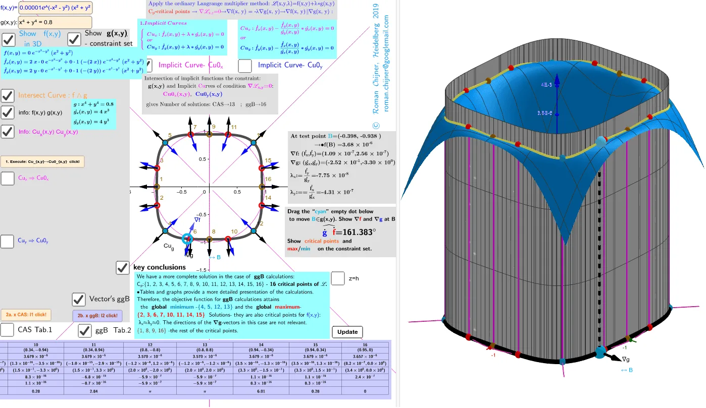
① 本范例通过三维图形直观演示拉格朗日乘数法在约束条件下求函数极值的过程,展示目标函数曲面与约束曲线(圆柱面)的交线以及最优点位置。② 核心数学概念包括多元函数极值、拉格朗日乘数法、梯度向量、约束曲线、切平面与法向量,以及偏导数方程组的求解。③ 作图要点:从构造摘要可见,使用了GeoGebra的CurveCartesian(参数曲线)、Surface(曲面)、Point(点)、Vector(向量)、Segment(线段)、Text(文本)等命令,并定义了目标函数f、约束函数g及其偏导数fx'、fy'、gx'、gy',通过梯度向量Vf、Vg和拉格朗日乘子l1、l2构建可视化,还包含按钮(button4等)和滑块(α)用于交互调节参数。④ 适合大学微积分或高等数学课程中讲解多元函数条件极值,也可用于数学建模或工程优化问题的教学演示,帮助学生理解拉格朗日乘数法的几何意义与代数求解过程。
GeoGebra 命令及参数
Simplify(Derivative[f, y, 1]) → fy'Simplify(Derivative[f, x, 1]) → fx'LeftSide(Cu_g) → gSimplify(Derivative[g, y, 1]) → gy'Simplify(Derivative[g, x, 1]) → gx'Point(Cu_g) → BVector(B, B + UnitVector[Vector[B, Dg]] / 3) → u_gVector(B, B + UnitVector[Vector[B, Df]] / 3) → u_fAngle(u_g, u_f) → αLaTeX(f, true) → text8aLaTeX(Cu_g, true) → text8bTextfield(f) → InputBox3Textfield(Cu_g) → InputBox4CurveCartesian(sqrt(cos(t)), (0.8 - cos(t)^(2))^(0.25), f(sqrt(cos(t)), (0.8 - cos(t)^(2))^(0.25)), t, (-π), π) → q1CurveCartesian((-sqrt(cos(t))), (0.8 - cos(t)^(2))^(0.25), f(sqrt(cos(t)), (0.8 - cos(t)^(2))^(0.25)), t, (-π), π) → q2CurveCartesian(sqrt(cos(t)), (-(0.8 - cos(t)^(2))^(0.25)), f(sqrt(cos(t)), (-(0.8 - cos(t)^(2))^(0.25))), t, (-π), π) → q1aCurveCartesian((-sqrt(cos(t))), (-(0.8 - cos(t)^(2))^(0.25)), f((-sqrt(cos(t))), (-(0.8 - cos(t)^(2))^(0.25))), t, (-π), π) → q2aTextfield(n) → InputBox5Element(l1, Indexmax1) → Amax1Element(l2, Indexmax2) → Amax2Element(l1, Indexmin1) → Amin1Element(l2, Indexmin2) → Amin2Element(l1f, Indexmax1) → Amax1_{3D}Element(l2f, Indexmax2) → Amax2_{3D}Element(l1f, Indexmin1) → Amin1_{3D}Element(l2f, Indexmin2) → Amin2_{3D}LaTeX(Amin2_{3D}, true, true) → text17Zip(ScientificText[a, 4], a, z(l2f)) → l2faZip(ScientificText[a, 4], a, z(l1f)) → l1faTableText(Append["N", 1…Length[l2]], Append["\fgcolor{red}{Cp}", l2], Append["\fgcolor{blue}{f}(\fgcolor{red}{C_p })", l2fa], Append["(\dot{f_x},\dot{f_y})", l2xy'_fa], Append["(\dot{g_x},\dot{g_y})", l2xy'_ga], Append["λ_x", lλ2ax], Append["λ_y", lλ2ay], Append["\widehat{\dot{g}\dot{f}} ", lα2], "c|_") → tTab2TableText(Append["N", 1…Length[l1]], Append["\fgcolor{red}{Cp}", l1], Append["\fgcolor{blue}{f}(\fgcolor{red}{C_p })", l1fa], Append["(\dot{f_x},\dot{f_y})", l1xy'_fa], Append["(\dot{g_x},\dot{g_y})", l1xy'_ga], Append["λ_x", lλ1ax], Append["λ_y", lλ1ay], Append["\widehat{\dot{g}\dot{f}} ", lα1], "c|_") → tTab1Segment(B, C) → f_1Text("∇f", Point[u_f, 1]) → text25fRotateText(text14, 90°) → text15Text("∇g", Point[u_g, 1]) → text25gSequence(If[lα1(i) ≟ 180°, 1, lα1(i) ≟ 0° ∨ lα1(i) ≟ 360°, 2, 3], i, 1, Length[l1]) → l1_αSurface(((-0.8^(0.25)) * (1 - sin(t)^(4))^(0.25)), (0.8^(0.25) * sin(t)), u, t, 0, (2 * π), u, 0, (4 * 10^(-6))) → g02Surface((0.8^(0.25) * (1 - sin(t)^(4))^(0.25)), (0.8^(0.25) * sin(t)), u, t, (-π), π, u, 0, (4 * 10^(-6))) → g01Surface(sqrt(cos(t)), (0.8 - cos(t)^(2))^(0.25), u, t, (-π), π, u, 0, (4 * 10^(-6))) → g1Surface((-sqrt(cos(t))), (0.8 - cos(t)^(2))^(0.25), u, t, (-π), π, u, 0, (4 * 10^(-6))) → g2Surface(sqrt(cos(t)), (-(0.8 - cos(t)^(2))^(0.25)), u, t, (-π), π, u, 0, (4 * 10^(-6))) → g1aSurface((-sqrt(cos(t))), (-(0.8 - cos(t)^(2))^(0.25)), u, t, (-π), π, u, 0, (4 * 10^(-6))) → g2aRemoveUndefined(Zip[If[(abs(x(A)) * 10^(15)) < 1 ∧ (abs(y(A)) * 10^(15)) < 1, b, (NaN, NaN)], A, l1xy'_f, b, l1]) → l1_{loc}RemoveUndefined(Zip[If[(abs(x(l2xy'_f(k))) * 10^(14)) < 1 ∧ (abs(y(l2xy'_f(k))) * 10^(14)) < 1, k, NaN], k, 1…Length[l2]]) → l2_{loc}NRemoveUndefined(Zip[If[(abs(x(l1xy'_f(k))) * 10^(14)) < 1 ∧ (abs(y(l1xy'_f(k))) * 10^(14)) < 1, k, NaN], k, 1…Length[l1]]) → l1_{loc}NRemoveUndefined(Sequence[If[lα1(i) ≟ 180°, i, NaN], i, 1, Length[l1]]) → l1_πNRemoveUndefined(Sequence[If[lα2(i) ≟ 180°, i, NaN], i, 1, Length[l2]]) → l2_πNRemoveUndefined(Sequence[If[lα2(i) ≟ 180°, l2(i), NaN], i, 1, Length[l2]]) → l2_πRemoveUndefined(Sequence[If[lα1(i) ≟ 180°, l1(i), NaN], i, 1, Length[l1]]) → l1_πRemoveUndefined(Sequence[If[lα2(i) ≟ 180°, l2f(i), NaN], i, 1, Length[l2]]) → l2_{π3D}RemoveUndefined(Sequence[If[lα1(i) ≟ 180°, l1f(i), NaN], i, 1, Length[l1]]) → l1_{π3D}Sequence(Text[i, l2(i) + (0.05, 0.1)], i, 1, lä2) → l2txtZip(Segment[a, b], a, l2, b, l2f) → l2segZip(Segment[a, b], a, l1, b, l1f) → l1segSequence(Text[i, l1(i) + (0.05, 0.1)], i, 1, lä1) → l1txtRemoveUndefined(Zip[If[(abs(x(A)) * 10^(14)) < 1 ∧ (abs(y(A)) * 10^(14)) < 1, b, (NaN, NaN)], A, l2xy'_f, b, l2]) → l2_{loc}RemoveUndefined(Zip[Vector[c, c + UnitVector[a] / 3], a, l1xy'_f, c, l1]) → lvec1_fRemoveUndefined(Zip[Vector[c, c + UnitVector[a] / 3], a, l1xy'_g, c, l1]) → lvec1_gRemoveUndefined(Zip[Vector[c, c + UnitVector[a] / 3], a, l2xy'_f, c, l2]) → lvec2_fRemoveUndefined(Zip[Vector[c, c + UnitVector[a] / 3], a, l2xy'_g, c, l2]) → lvec2_gRemoveUndefined(Zip[If[(abs(x(A)) * 10^(14)) < 1 ∧ (abs(y(A)) * 10^(14)) < 1, b, (NaN, NaN)], A, l2xy'_f, b, l2f]) → l2_{loc3D}RemoveUndefined(Zip[If[(abs(x(A)) * 10^(14)) < 1 ∧ (abs(y(A)) * 10^(14)) < 1, b, (NaN, NaN)], A, l1xy'_f, b, l1f]) → l1_{loc3D}Simplify(fy'(x, y) - (gy'(x, y) * fx'(x, y) / gx'(x, y))) → Cu_yfSimplify(fx'(x, y) - (gx'(x, y) * fy'(x, y) / gy'(x, y))) → Cu_xfTextfield(txtCu01_x) → InputBox1Textfield(txtCu01_y) → InputBox2
AI 绘图提示语参考
绘制一个三维曲面,该曲面由函数f(x,y)定义,同时包含一个约束曲面g(x,y)。首先绘制f(x,y)的等高线,然后绘制g(x,y)的等高线,接着找到f(x,y)和g(x,y)的交点,标记出这些交点,并在这些点处绘制梯度向量。最后,通过调整参数α,观察梯度向量之间的夹角变化,理解拉格朗日乘数法在条件极值问题中的应用。
以上提示语为根据原始绘图命令整理而来,仅供参考。