
用两种方法求解棘手极限
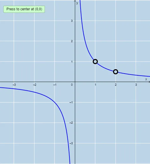
几何画板及绘图内容加载中,请稍等……
本范例通过两种方法求解一个棘手的极限问题。核心数学概念包括极限、函数和不等式。使用了GeoGebra中的Root、Intersection、Length、Sequence、Limit等命令。适合高中数学教学和学习。
GeoGebra 命令及参数
Root(Denominator[r]) → A, B, CIntersection(rootsd, rootsm) → commonrootsLength(commonroots) → numberofholesSequence(x = x(Element[commonroots, i]), i, 1, numberofholes, 1) → linesSequence(x(Element[commonroots, i]), i, 1, numberofholes, 1) → xvalsSequence((Element[xvals, i], r(Element[xvals, i])), i, 1, numberofholes, 1) → holesSequence(Limit[r, Element[xvals, i]], i, 1, numberofholes, 1) → list1Sequence((Element[xvals, i], Element[list1, i]), i, 1, numberofholes, 1) → list2Limit(r, Infinity) → aLimit(r, -Infinity) → bTextfield(n) → InputBox1Textfield(d) → InputBox2PartialFractions(r) → pSequence((Element[xvals, i], Element[list1, i]), i, 1, numberofholes, 1) → l1
AI 绘图提示语参考
绘制一个有理函数的极限分析图。首先在坐标系中画出函数图像,重点关注函数的可去间断点——即分母为零但分子也为零的x坐标位置。用虚线在这些x值处画垂线标记间断点位置,并在每个间断点处标注函数趋近的极限值。同时在图像右侧或上方显示函数在正无穷和负无穷远处的极限值。整体呈现函数图像及其关键极限特征,帮助理解极限的不同计算方法。
以上提示语为根据原始绘图命令整理而来,仅供参考。