
离心率证明
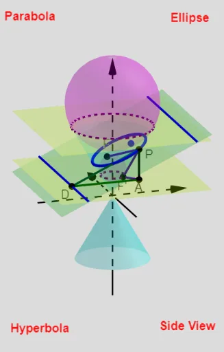
几何画板及绘图内容加载中,请稍等……
①本范例演示了离心率在二维平面上等于距离比,在三维空间中等于平面与锥面角度正弦比的现象;②涉及核心数学概念包括圆、锥、圆锥截面、椭圆、双曲线、抛物线、整数、全等、二次方程、勾股定理、方差;③作图要点:使用了Line(线段)、AngularBisector(角平分线)、Intersect(交点)、OrthogonalLine(垂线)、Circle(圆)、Cone(锥)、Sphere(球)、CurveCartesian(笛卡尔曲线)、Segment(线段)、IntersectPath(路径交点)、Plane(平面)、Ray(射线)、Angle(角度)等GeoGebra命令/对象;④适合高中及以上数学学习者,用于理解离心率与几何图形的关系。
GeoGebra 命令及参数
If(abs(Z_{int}) > E_{psilon} ∧ abs(sin(θ_{plane-r})) < 0.9999, true, false) → S_{tandard}Line(P_{z}, (1, 0, z(P_{z}) + tan(θ_{plane-r}))) → L_{plane}Line((0, 0, 0), (r_{cone}, 0, 5)) → L_{cone-r}AngularBisector(L_{plane}, L_{cone-r}) → L_{bis-1}, L_{bis-2}Intersect(L_{bis-1}, zAxis) → P_{circle-1}OrthogonalLine(P_{circle-1}, L_{plane}, x = 0) → L_{perp-1}If(S_{tandard}, Intersect[L_{perp-1}, L_{plane}]) → F_{1}OrthogonalLine(P_{circle-1}, L_{cone-r}, x = 0) → L_{perp-1a}Intersect(L_{perp-1a}, L_{cone-r}) → P_{horz-1}Line(P_{horz-1}, xAxis) → L_{horz-1}Intersect(L_{horz-1}, L_{plane}) → P_{d1}Intersect(L_{bis-2}, zAxis) → P_{circle-2}OrthogonalLine(P_{circle-2}, L_{plane}, x = 0) → L_{perp-2}If(S_{tandard}, Intersect[L_{perp-2}, L_{plane}]) → F_{2}If(S_{tandard}, Distance[P_{circle-2}, L_{plane}], sqrt(-1)) → r_{2}Circle(P_{circle-2}, r_{2}, y = 0) → C_{circle-2}If(S_{tandard}, Distance[P_{circle-1}, L_{plane}], sqrt(-1)) → r_{1}Circle(P_{circle-1}, r_{1}, y = 0) → C_{circle-1}Line((0, 0, 0), ((-r_{cone}), 0, 5)) → L_{cone-l}Cone((0, 0, 5), (0, 0, 0), r_{cone}) → C_{cone-top}, C_1, C_3Cone((0, 0, -5), (0, 0, 0), r_{cone}) → C_{cone-bot}, c, C_2Intersect(L_{plane}, L_{cone-r}) → P_{r}Intersect(L_{plane}, L_{cone-l}) → P_{l}Sphere(P_{circle-1}, r_{1}) → s_{1}Sphere(P_{circle-2}, r_{2}) → s_{2}OrthogonalLine(P_{circle-2}, L_{cone-r}, x = 0) → L_{perp-2a}Intersect(L_{perp-2a}, L_{cone-r}) → P_{horz-2}Line(P_{horz-2}, xAxis) → L_{horz-2}Intersect(L_{horz-2}, L_{plane}) → P_{d2}CurveCartesian((((r(θ) * sin(θ)) * cos(θ_{plane-r})) * sgn(Z_{int+e})) + x(F_{1}), (r(θ) * cos(θ)), (((r(θ) * sin(θ)) * sin(θ_{plane-r})) * sgn(Z_{int+e})) + z(F_{1}), θ, 0, 6.3) → C_{conic}If(S_{tandard}, C_{conic}) → C_{conic-disp}If(¬S_{tandard}, Line[(0, 0, 0), (cot(θ_{plane-r}), (-y_{deg}), 1)]) → L_{degm}If(¬S_{tandard}, Line[(0, 0, 0), (cot(θ_{plane-r}), y_{deg}, 1)]) → L_{degp}If(S_{tandard}, Line[P_{d1}, yAxis]) → L_{d1}If(S_{tandard}, Line[P_{d2}, yAxis]) → L_{d2}If(S_{tandard}, C_{conic}) → aOrthogonalLine(P, L_{d1}, space) → L_{PD-line}Intersect(L_{PD-line}, L_{d1}) → DSegment(P, D) → L_{PD}Segment(P, F_{1}) → L_{PF}IntersectPath(P_{plane1}, s_{1}) → C_{s1-plane1}IntersectPath(P_{plane2}, s_{2}) → C_{plane2-s2}OrthogonalLine(P, P_{plane1}) → L_{P-plane1}Intersect(L_{P-plane1}, P_{plane1}) → ASegment(P, A) → L_{PA}Segment(D, A) → L_{DA}Plane(F_{1}, P, A) → P_{PFA}Line(P, (0, 0, 0)) → L_{P-0}Intersect(L_{P-0}, P_{plane1}) → F'Segment(P, F') → L_{PF'}Segment(F', A) → L_{F'A}Ray(D_g, (100, y(D_g))) → fCircle(D_g, L_{DA}) → dIntersect(d, f) → A_{g-plane},Circle(A_{g-plane}, L_{PA}) → hRay(A_{g-plane}, (x(A_{g-plane}), 100)) → gIntersect(h, g) → P_{g-plane},Segment(D_g, A_{g-plane}) → iSegment(A_{g-plane}, P_{g-plane}) → sSegment(P_{g-plane}, D_g) → tAngle(A_{g-plane}, D_g, P_{g-plane}) → θ_{plane}Ray(F'_g, (100, y(F'_g))) → jCircle(F'_g, L_{F'A}) → kIntersect(k, j) → A_{g-cone},Ray(A_{g-cone}, (x(A_{g-cone}), 100)) → lCircle(F'_g, L_{PF'}) → pIntersect(p, l) → P_{g-cone},Segment(F'_g, A_{g-cone}) → mSegment(A_{g-cone}, P_{g-cone}) → nSegment(P_{g-cone}, F'_g) → qAngle(A_{g-cone}, F'_g, P_{g-cone}) → θ_{cone}
AI 绘图提示语参考
画一个二维平面上的椭圆和三维空间中的圆锥,展示离心率与距离比的关系。首先,在平面上画一条直线和一个角度平分线,交点处画圆。然后,从圆心向平面和圆锥母线作垂线,得到焦点和与圆锥的交点。接着,画出圆锥和球体,并显示与平面的交线。最后,用曲线工具画出圆锥截面,并标出关键点和线段,展示离心率与几何形状的关系。
以上提示语为根据原始绘图命令整理而来,仅供参考。