圆锥曲线离心率的几何可视化与作图演示

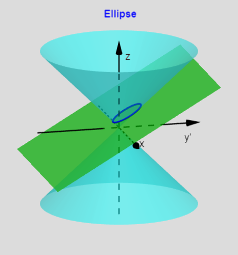
几何画板及绘图内容加载中，请稍等……

2021-03-19 20:39

该范例通过圆锥与平面相交的空间几何关系，展示离心率 e 如何刻画椭圆、抛物线与双曲线等圆锥曲线的“伸展程度”。核心数学概念包括：离心率（eccentricity）的几何意义、圆锥曲线的生成（平面截圆锥）、以及与角度相关的几何关系（如角平分线与垂线构造）。作图要点是把若干关键方向角（如 θ_{plane}、θ_{cone} 及其变体）与对应半径/距离量（如 r、r_{cone}、r_p 等）组织到一套参数几何框架中：使用 Line 画直线，利用 If 进行条件分支以选择不同构型，借助 AngularBisector 构造角平分线、OrthogonalLine 与（多处）L_{perp-1} 类对象建立垂线关系；再用 Intersect/IntersectPath 确定相交点与截线轨迹；通过 Cone 与 Sphere 进行三维主体建模，并用 CurveCartesian 表示由参数映射得到的曲线；最后用 Circle 与 Segment 补充必要的圆与线段约束，形成可观察的截交曲线与辅助几何元素（如 CornerThreeD、Corner1、CornerThreeD 相关角点对象与一系列点/线标签）。适合高中到大学的解析几何与立体几何教学，尤其适用于讲授圆锥曲线生成机理、离心率直观理解与参数化建模的课堂演示或自学练习。

GeoGebra 命令及参数

Line((0, 0, 0), (0, r_{cone}, 5)) → L_{cone-r}
If(Z_{int} ≠ 0 ∧ abs(sin(θ_{plane-r})) < 0.9999, true, false) → S_{tandard}
Line(P_{z}, (0, 1, z(P_{z}) + tan(θ_{plane-r}))) → L_{plane}
AngularBisector(L_{plane}, L_{cone-r}) → L_{bis-1}, L_{bis-2}
If(e_{s} ≟ 1, (0, 0, Z_{int} / 2), Intersect[L_{bis-1}, zAxis]) → P_{circle-1}
OrthogonalLine(P_{circle-1}, L_{plane}, y = 0) → L_{perp-1}
If(e_{s} ≟ 1, F_{1par}, Intersect[L_{perp-1}, L_{plane}]) → F_{1}
If(e_{s} > 1, asin(1 / e_{s}), 1) → A_{symp1}
If(S_{tandard}, L_{SLR}^(2), 0) → C_{c}
If(S_{tandard}, ((2 * L_{SLR}) * e_{s}), 0) → C_{y}
CornerThreeD(-1, 11) → Corner1
OrthogonalLine(P_{circle-1}, L_{cone-r}, y = 0) → L_{perp-1a}
Intersect(L_{perp-1a}, L_{cone-r}) → P_{horz-1}
Line(P_{horz-1}, yAxis) → L_{horz-1}
Intersect(L_{horz-1}, L_{plane}) → P_{d1}
Line((0, D_{ist}(y(P_{d1}))), xAxis) → L_{d1-g}
Line(P_{g}, yAxis) → L_{Pg}
Intersect(L_{Pg}, L_{d1-g}) → D_1
Segment(P_{g}, F_{1g}) → L_{PF-g}
Segment(P_{g}, D_1) → L_{PD-g}
Intersect(L_{bis-2}, zAxis) → P_{circle-2}
OrthogonalLine(P_{circle-2}, L_{plane}, y = 0) → L_{perp-2}
Intersect(L_{perp-2}, L_{plane}) → F_{2}
If(S_{tandard}, Distance[P_{circle-2}, L_{plane}], sqrt(-1)) → r_{2}
If(S_{tandard}, Distance[P_{circle-1}, L_{plane}], sqrt(-1)) → r_{1}
Line((0, 0, 0), (0, (-r_{cone}), 5)) → L_{cone-l}
Cone((0, 0, 5), (0, 0, 0), r_{cone}) → C_{cone-top}, C_1, C_3
Cone((0, 0, -5), (0, 0, 0), r_{cone}) → C_{cone-bot}, c, C_2
Intersect(L_{plane}, L_{cone-r}) → P_{r}
Intersect(L_{plane}, L_{cone-l}) → P_{l}
Sphere(P_{circle-1}, r_{1}) → s_{1}
Sphere(P_{circle-2}, r_{2}) → s_{2}
OrthogonalLine(P_{circle-2}, L_{cone-r}, y = 0) → L_{perp-2a}
Intersect(L_{perp-2a}, L_{cone-r}) → P_{horz-2}
Line(P_{horz-2}, yAxis) → L_{horz-2}
Intersect(L_{horz-2}, L_{plane}) → P_{d2}
CurveCartesian((r(θ) * cos(θ)), ((r(θ) * sin(θ)) * sgn(Z_{int})), θ, 0, 6.3) → C_{conic-g}
CurveCartesian((r(θ) * cos(θ)), (((r(θ) * sin(θ)) * cos(θ_{plane-r})) * sgn(Z_{int})) + y(F_{1}), (((r(θ) * sin(θ)) * sin(θ_{plane-r})) * sgn(Z_{int})) + z(F_{1}), θ, 0, 6.3) → C_{conic}
IntersectPath(P_{plane1}, s_{1}) → C_{plane1-s1}
IntersectPath(P_{plane2}, s_{2}) → C_{plane2-s2}
Circle(P_{circle-1}, r_{1}, x = 0) → C_{circle-1}
Circle(P_{circle-2}, r_{2}, x = 0) → C_{circle-2}
If(x(Corner1) ≟ -1, 1, If[x(Corner1) ≟ 0, 3, 2]) → View
If(S_{tandard} ≠ 0 ∧ D ≤ 3, If[PointP < 0, "Show", " Hide"]) → textShowHide
If(D ≤ 3, If[PointP < 0, " Point P", " Point P"], "Point P") → textP
CurveCartesian((r(θ) * cos(θ)), (((r(θ) * sin(θ)) * cos(θ_{plane-r})) * sgn(Z_{int})) + y(F_{1}), (((r(θ) * sin(θ)) * sin(θ_{plane-r})) * sgn(Z_{int})) + z(F_{1}), θ, A_{symp1m}, A_{symp1p}) → C_{conic1}
CurveCartesian((r(θ) * cos(θ)), (((r(θ) * sin(θ)) * cos(θ_{plane-r})) * sgn(Z_{int})) + y(F_{1}), (((r(θ) * sin(θ)) * sin(θ_{plane-r})) * sgn(Z_{int})) + z(F_{1}), θ, A_{symp2m}, A_{symp2p}) → C_{conic2}
Line((0, 0), ((-A_{rslope}), 1)) → L_{degm-g}
Line((0, 0, 0), ((-x_{deg}), cot(θ_{plane-r}), 1)) → L_{degm}
Line((0, 0), (A_{rslope}, 1)) → L_{degp-g}
Line((0, 0, 0), (x_{deg}, cot(θ_{plane-r}), 1)) → L_{degp}
If(θ_{plane} ≠ 90, z = Z_{int} + (tan(θ_{plane-r}) * y), y = 0) → P_{plane}
Line(P_{d1}, xAxis) → L_{d1}
Line((0, D_{ist}(y(P_{d2}))), xAxis) → L_{d2-g}
Line(P_{d2}, xAxis) → L_{d2}
If(e_{s} ≤ 1, "+", "-") → signQ
If(Z_{int} ≤ 0, "+", "-") → signL
If(S_{tandard}, If[e_{s} ≟ 0, " Circle ", e_{s} < 1, " Ellipse ", e_{s} ≟ 1, " Parabola ", "Hyperbola"], e_{s} < 1, " Point ", e_{s} ≟ 1, " Line ", "Two Lines") → ConicName

AI 绘图提示语参考

根据圆锥与截平面的相交来展示二次曲线的离心率决定形状：建立一对圆锥（上、下指向同一顶点）与两条关键平面（一个由平面倾角控制），同时设置空间参考轴与若干夹角控制量。用角平分线与垂线关系辅助确定圆周交点所在的圆心，然后构造与该圆心到平面距离相关的两个半径。进一步在空间中以截平面与圆锥的交线作为约束，生成两条由参数方程驱动的曲线表示椭圆/双曲线（当离心率小于或大于 1 时采用不同分支），再在三维空间中叠加截取轨迹以强调曲线来自“切片圆锥”。

以上提示语为根据原始绘图命令整理而来，仅供参考。