
y=mx+b: An Investigation
Loading the math board and drawing, please wait…
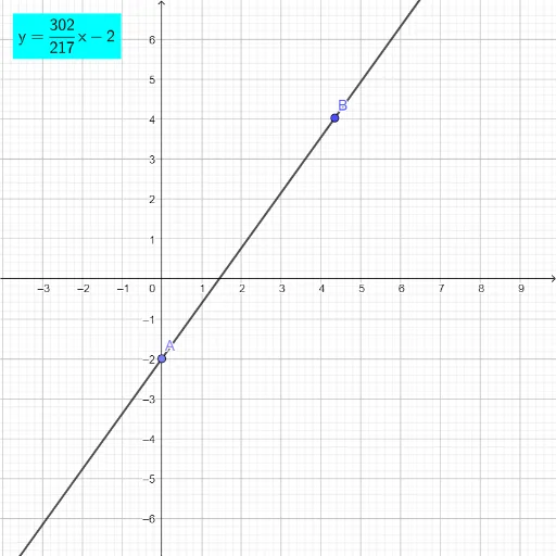
① This GeoGebra example dynamically explores the linear function y=mx+b by allowing users to adjust the slope m and y-intercept b, observing how the graph changes in real time along with the displayed equation, slope value, and key point coordinates. ② Core mathematical concepts include linear functions, slope, intercept, function graphs, the relationship between equation and line, as well as extensions to equilateral triangles, histograms, and linear regression. ③ Construction details: using GeoGebra commands Point to create points A and B, Line to construct line f, Slope to compute slope a, FractionText to display the slope as a fraction, Text for labels, and If for conditional display, resulting in dynamic text objects text1, text2, and text3. ④ Suitable for middle and high school students learning algebra and function graphing, and for teachers demonstrating how parameter changes affect linear function graphs.
GeoGebra Commands & Parameters
Point(yAxis) → ALine(A, B) → fSlope(f) → aFractionText(a) → text1Text(b) → text2If(a ≟ -1 ∨ a ≟ 0 ∨ a ≟ 1, LaTeX[f], LaTeX["y=" + text1 + "x" + (If[b > 0, "+", ""]) + (If[b ≟ 0, "", text2])]) → text3
AI Drawing Prompt Reference
Draw a line y=mx+b, where m is the slope and b is the y-intercept. Start by taking a point A on the y-axis, then draw a line f through A and another point B. Calculate the slope a of line f and display it as a fraction. Then show the values of slope a and y-intercept b. Finally, dynamically display the equation of the line as y=ax+b or y=ax±b based on the values of a and b.
The prompt above was compiled from the original drawing commands and is for reference only.