
Volumes of Revolution Using Shells
Loading the math board and drawing, please wait…
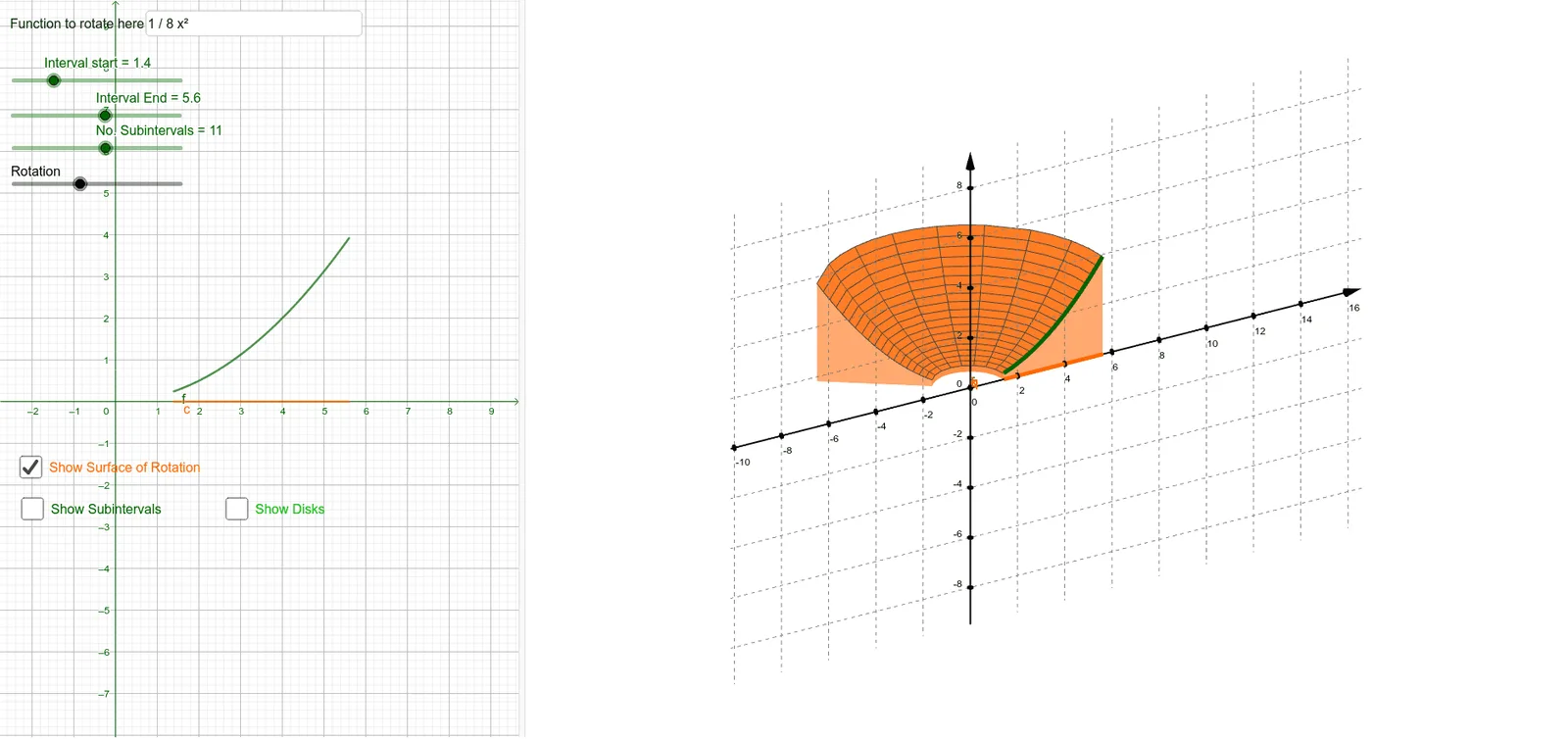
This example demonstrates calculating the volume of a solid of revolution using the shell method. It involves core math concepts like integral calculus and volume computation. Constructed with GeoGebra commands such as Sequence, Textfield, CurveCartesian, and Surface. Ideal for high school students and calculus learners.
GeoGebra Commands & Parameters
Sequence(Segment[(k, f(k), 0), (k + d, f(k), 0)], k, a, b - d, d) → l3Textfield(g) → FunctionCurveCartesian(t, f(t), t, a, b) → jSequence(Surface[CurveCartesian[t, f(k), t, k, k + d], theta, yAxis], k, a, b - d, d) → l1Sequence(Surface[CurveCartesian[k, t, t, 0, g(k)], theta, yAxis], k, a, b, d) → l6Surface(j, theta, yAxis) → lCurveCartesian(t, 0, t, a, b) → cSequence(Segment[(k, 0, 0), (k, f(k), 0)], k, a, b, d) → l4Surface(c, theta, yAxis) → kCurveCartesian(b, t, t, 0, g(b)) → mSurface(m, theta, yAxis) → oCurveCartesian(a, t, t, 0, g(a)) → pSurface(p, theta, yAxis) → q
AI Drawing Prompt Reference
Draw a demonstration of calculating the volume of a solid of revolution, featuring a function curve and its rotated surface, with dashed line segments indicating the integral interval, and multiple shell-like surfaces stacked to show the volume calculation process, presenting the geometric relationship between the solid and shells to help understand the shell method for volume computation.
The prompt above was compiled from the original drawing commands and is for reference only.