
Volumes of Revolution: Disk vs. Shell Method Comparison
Loading the math board and drawing, please wait…
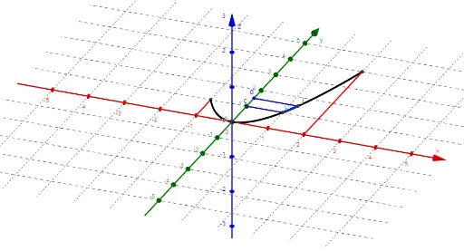
This GeoGebra example dynamically demonstrates two classic methods for computing volumes of revolution: the Disk Method and the Shell Method. It revolves a planar region (bounded by function curves, coordinate axes, and boundary lines) around an axis to generate a 3D solid, then approximates the volume using perpendicular disk slices and parallel shell slices, visually comparing the geometric meaning of the two integral formulas. Core mathematical concepts include definite integrals for volume, solids of revolution, function graphs, trigonometric functions, and quadratic equations. Construction highlights: uses CurveCartesian to plot curves, Ray and Segment to define the rotation axis and boundaries, Surface to generate the revolved surface, Intersect to find intersection points, Textfield for parameter input, and sliders (e.g., k_x, k_y) to dynamically adjust the axis position or function parameters, with Invert for view toggling. Suitable for senior high school or introductory college calculus, helping students grasp the derivation and geometric intuition behind volume integral formulas.
GeoGebra Commands & Parameters
Textfield(f) → FunctionTextfield(a) → Textfeld2Textfield(b) → Textfeld3CurveCartesian(t, (f(t) * cos(φ)), (f(t) * sin(φ)), t, a, b) → k_xRay((0, c), Vector[(1, 0)]) → g_1Intersect(f, g_1, (1, f(1))) → IRay((0, d), Vector[(1, 0)]) → g_2Intersect(f, g_2, (d, f(d))) → JCurveCartesian((t * cos(ϕ)), f(t), (t * sin(ϕ)), t, x(I), x(J)) → k_yCurveCartesian(t, f(t), 0, t, -5, 5) → kTextfield(c) → Textfeld4Textfield(d) → Textfeld5Segment(A, G) → s_1Segment(B, F) → s_2Surface(u, (f(u) * cos(w)), (f(u) * sin(w)), u, a, b, w, 0, φ) → f_xSurface((uu * cos(ww)), f(uu), (uu * sin(ww)), uu, x(I), x(J), ww, 0, ϕ) → f_yInvert(f) → f_uSegment(C, I) → s_3Segment(D, J) → s_4CurveCartesian(x(B), t, t, y(B), f(x(B))) → LineCapRightCurveCartesian(x(A), t, t, y(A), f(x(A))) → LineCapLeftSurface(x(A), y(A) + ((s * (f(x(A)) - y(A))) * cos(t)), ((s * (f(x(A)) - y(A))) * sin(t)), s, 0, 1, t, 0, φ) → CapLeftSurface(x(B), y(B) + ((s * (f(x(B)) - y(B))) * cos(t)), ((s * (f(x(B)) - y(B))) * sin(t)), s, 0, 1, t, 0, φ) → CapRightCurveCartesian(t, y(C), t, x(C), f_u(y(C))) → LineCapBottomCurveCartesian(t, y(D), t, x(D), f_u(y(D))) → LineCapTop
AI Drawing Prompt Reference
Create a dynamic illustration showing two methods for calculating volumes of revolution. Begin by drawing a planar region bounded by function curves, coordinate axes, and boundary lines, then revolve it around an axis to generate a 3D solid. Approximate the volume using perpendicular disk slices and parallel shell slices to visually compare the geometric meaning of the two integral formulas. Include function curves, a rotation axis, the generated surface, intersection points, parameter input fields, and sliders for dynamic adjustment of the axis position or function parameters.
The prompt above was compiled from the original drawing commands and is for reference only.