
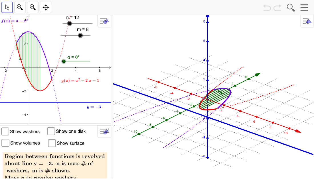
Volumes of Revolution between Two Quadratics Rotated around y=-3
Loading the math board and drawing, please wait…
This example demonstrates the calculation of the volume of revolution formed by rotating two quadratic functions around the line y=-3 using the washer method. Key math concepts include volumes of revolution, washer method, and integral calculus. GeoGebra commands used are Sequence, Rotate, RectangleSum, Surface, Polygon, and Integral. Suitable for high school and above students learning calculus volume calculations and geometric visualization.
GeoGebra Commands & Parameters
Sequence(Polygon[(-1 + (k * h), g(-1 + ((k + p) * h))), (-1 + ((k + 1) * h), g(-1 + ((k + p) * h))), (-1 + ((k + 1) * h), f(-1 + ((k + p) * h))), (-1 + (k * h), f(-1 + ((k + p) * h)))], k, 0, m - 1) → RectanglesRotate(Rectangles, (-α), a) → Rectangles'RectangleSum(A, -1, -1 + (m * h), m, p) → VolWashersSurface(-1 + (DK * h), -3 + ((u + 3) * cos(β)), ((u + 3) * sin(β)), u, g(-1 + ((DK + p) * h)), f(-1 + ((DK + p) * h)), β, 0, α) → SideLeft1Surface(-1 + ((DK + 1) * h), -3 + ((u + 3) * cos(β)), ((u + 3) * sin(β)), u, g(-1 + ((DK + p) * h)), f(-1 + ((DK + p) * h)), β, 0, α) → SideRight1Surface(u, -3 + ((f(-1 + ((DK + p) * h)) + 3) * cos(β)), ((f(-1 + ((DK + p) * h)) + 3) * sin(β)), u, -1 + (DK * h), -1 + ((DK + 1) * h), β, 0, α) → Outer1Surface(u, -3 + ((g(-1 + ((DK + p) * h)) + 3) * cos(β)), ((g(-1 + ((DK + p) * h)) + 3) * sin(β)), u, -1 + (DK * h), -1 + ((DK + 1) * h), β, 0, α) → Inner1Polygon((-1 + (DK * h), g(-1 + ((DK + p) * h))), (-1 + ((DK + 1) * h), g(-1 + ((DK + p) * h))), (-1 + ((DK + 1) * h), f(-1 + ((DK + p) * h))), (-1 + (DK * h), f(-1 + ((DK + p) * h)))) → Rectangle1, b, c, d, eRotate(Rectangle1, (-α), a) → Rectangle1'Integral((π * ((f(x) + 3)^(2) - (g(x) + 3)^(2))), -1, 2) → VolIntegRotate(f_1, (-α), a) → iRotate(g_1, (-α), a) → jSurface(u, -3 + ((f(u) + 3) * cos(β)), ((f(u) + 3) * sin(β)), u, -1, 2, β, 0, (2 * π)) → OuterSurface(u, -3 + ((g(u) + 3) * cos(β)), ((g(u) + 3) * sin(β)), u, -1, 2, β, 0, (2 * π)) → InnerSequence(Surface[-1 + ((k + u) * h), -3 + ((3 + f(-1 + ((k + p) * h))) * cos(β)), ((3 + f(-1 + ((k + p) * h))) * sin(β)), u, 0, 1, β, 0, α], k, 0, m - 1) → OutersSequence(Surface[-1 + ((k + u) * h), -3 + ((3 + g(-1 + ((k + p) * h))) * cos(β)), ((3 + g(-1 + ((k + p) * h))) * sin(β)), u, 0, 1, β, 0, α], k, 0, m - 1) → InnersSequence(Surface[-1 + (k * h), -3 + ((3 + (v * g(-1 + ((k + p) * h))) + ((1 - v) * f(-1 + ((k + p) * h)))) * cos(β)), ((3 + (v * g(-1 + ((k + p) * h))) + ((1 - v) * f(-1 + ((k + p) * h)))) * sin(β)), v, 0, 1, β, 0, α], k, 0, m - 1) → SidesLeftSequence(Surface[-1 + ((k + 1) * h), -3 + ((3 + (v * g(-1 + ((k + p) * h))) + ((1 - v) * f(-1 + ((k + p) * h)))) * cos(β)), ((3 + (v * g(-1 + ((k + p) * h))) + ((1 - v) * f(-1 + ((k + p) * h)))) * sin(β)), v, 0, 1, β, 0, α], k, 0, m - 1) → SidesRight