
Volume of Revolution Example by John Stenger
Loading the math board and drawing, please wait…
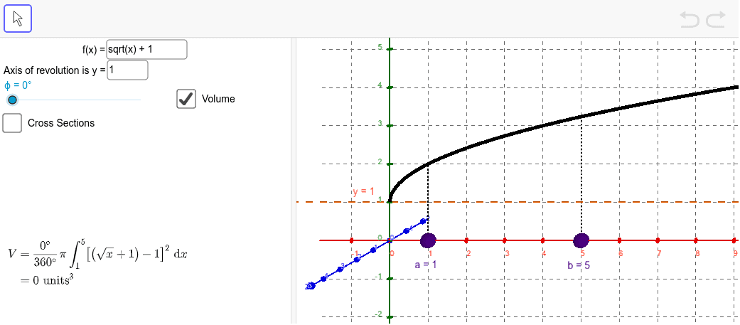
This example demonstrates how to calculate the volume of a solid of revolution using the disk method. The core mathematical concepts involve calculus, geometry, and function transformations. Construction involves GeoGebra commands such as Point, Intersect, Surface, and Polygon. Suitable for high school students or college freshmen learning calculus and solid geometry.
GeoGebra Commands & Parameters
Point(xAxis) → APoint(xAxis) → BIntersect(f, b, (5, 3.23606797749979)) → DIntersect(f, a, (1, 2)) → CSegment(A, C) → dSegment(B, D) → eSequence((x(A) + (k * Δx), (f(x(A) + (k * Δx)) * cos(ϕ)), (f(x(A) + (k * Δx)) * sin(ϕ))), k, 0, n - 1) → tracepointsTextfield(f) → inputBox1Textfield(axis) → inputBox2Sequence(Surface[x(A) + (u * Δx), axis + ((f(x(A) + (k * Δx)) - axis) * cos(v)), ((f(x(A) + (k * Δx)) - axis) * sin(v)), u, k, k + 1, v, 0, ϕ], k, 0, n - 1) → surfacesSurface(x(A) + (u * Δx), axis + ((f(x(A) + ((i - 1) * Δx)) - axis) * cos(v)), ((f(x(A) + ((i - 1) * Δx)) - axis) * sin(v)), u, i - 1, i, v, 0, ϕ) → surface_{i}Sequence(Polygon[(x(A) + (k * Δx), axis), (x(A) + (k * Δx), f(x(A) + (k * Δx))), (x(A) + ((k + 1) * Δx), f(x(A) + (k * Δx))), (x(A) + ((k + 1) * Δx), axis)], k, 0, n - 1) → rectanglesPolygon((x(A) + ((i - 1) * Δx), axis, 0), (x(A) + ((i - 1) * Δx), axis + ((f(x(A) + ((i - 1) * Δx)) - axis) * cos(ϕ)), ((f(x(A) + ((i - 1) * Δx)) - axis) * sin(ϕ))), (x(A) + (i * Δx), axis + ((f(x(A) + ((i - 1) * Δx)) - axis) * cos(ϕ)), ((f(x(A) + ((i - 1) * Δx)) - axis) * sin(ϕ))), (x(A) + (i * Δx), axis, 0)) → face_{i}, c, j, k, lSequence(CircumcircleSector[(x(A) + (k * Δx), f(x(A) + ((i - 1) * Δx)), 0), (x(A) + (k * Δx), axis + ((f(x(A) + ((i - 1) * Δx)) - axis) * cos(ϕ / 2)), ((f(x(A) + ((i - 1) * Δx)) - axis) * sin(ϕ / 2))), (x(A) + (k * Δx), axis + ((f(x(A) + ((i - 1) * Δx)) - axis) * cos(ϕ)), ((f(x(A) + ((i - 1) * Δx)) - axis) * sin(ϕ)))], k, i - 1, i) → endcaps_{i}Sequence(Polygon[(x(A) + ((k - 1) * Δx), axis, 0), (x(A) + ((k - 1) * Δx), axis + ((f(x(A) + ((k - 1) * Δx)) - axis) * cos(ϕ)), ((f(x(A) + ((k - 1) * Δx)) - axis) * sin(ϕ))), (x(A) + (k * Δx), axis + ((f(x(A) + ((k - 1) * Δx)) - axis) * cos(ϕ)), ((f(x(A) + ((k - 1) * Δx)) - axis) * sin(ϕ))), (x(A) + (k * Δx), axis, 0)], k, 1, n) → facesSequence(CircumcircleSector[(x(A) + (k * Δx), f(x(A) + (k * Δx)), 0), (x(A) + (k * Δx), axis + ((f(x(A) + (k * Δx)) - axis) * cos(ϕ / 2)), ((f(x(A) + (k * Δx)) - axis) * sin(ϕ / 2))), (x(A) + (k * Δx), axis + ((f(x(A) + (k * Δx)) - axis) * cos(ϕ)), ((f(x(A) + (k * Δx)) - axis) * sin(ϕ)))], k, 0, n - 1) → endcaps_{left}Sequence(CircumcircleSector[(x(A) + (k * Δx), f(x(A) + ((k - 1) * Δx)), 0), (x(A) + (k * Δx), axis + ((f(x(A) + ((k - 1) * Δx)) - axis) * cos(ϕ / 2)), ((f(x(A) + ((k - 1) * Δx)) - axis) * sin(ϕ / 2))), (x(A) + (k * Δx), axis + ((f(x(A) + ((k - 1) * Δx)) - axis) * cos(ϕ)), ((f(x(A) + ((k - 1) * Δx)) - axis) * sin(ϕ)))], k, 1, n) → endcaps_{right}Polygon((x(A) + ((i - 1) * Δx), axis), (x(A) + ((i - 1) * Δx), f(x(A) + ((i - 1) * Δx))), (x(A) + (i * Δx), f(x(A) + ((i - 1) * Δx))), (x(A) + (i * Δx), axis)) → rectangle_{i}, g, m, p, qSequence(Cylinder[(x(A) + (k * Δx), axis, 0), (x(A) + ((k + 1) * Δx), axis, 0), f(x(A) + (k * Δx)) - axis], k, 0, n - 1) → cylindersSurface(t, axis + ((f(t) - axis) * cos(u)), ((f(t) - axis) * sin(u)), t, x(A), x(B), u, 0, ϕ) → surface_{whole}CircumcircleSector((x(A), f(x(A)), 0), (x(A), axis + ((f(x(A)) - axis) * cos(ϕ / 2)), ((f(x(A)) - axis) * sin(ϕ / 2))), (x(A), axis + ((f(x(A)) - axis) * cos(ϕ)), ((f(x(A)) - axis) * sin(ϕ)))) → endcap_{A}CircumcircleSector((x(B), f(x(B)), 0), (x(B), axis + ((f(x(B)) - axis) * cos(ϕ / 2)), ((f(x(B)) - axis) * sin(ϕ / 2))), (x(B), axis + ((f(x(B)) - axis) * cos(ϕ)), ((f(x(B)) - axis) * sin(ϕ)))) → endcap_{B}
AI Drawing Prompt Reference
Draw a function graph and mark two points on it. Construct two line segments using these points and the intersection points of the function graph. Use these line segments and the function graph to draw a series of rectangles and circular arc sectors, simulating the cross-sections and lateral surfaces of a solid of revolution. Finally, combine these shapes to illustrate the volume calculation process of the solid, including the base, lateral surface, and top.
The prompt above was compiled from the original drawing commands and is for reference only.