Volume by the Shell Method: Nested Cylinders Visualization

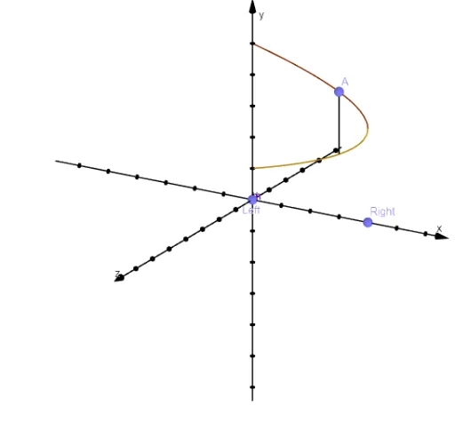
This example illustrates the shell method for computing the volume of a solid of revolution by representing it as a set of nested thin cylinders (shells). Visually, it shows how a region bounded by a curve over an interval rotates around a specified line, producing a volume that can be approximated by summing cylinder volumes whose radius and height vary with position, and then becomes exact in the limiting sense. Key concepts include volume of revolution, the shell method, variable radius/height geometry, interval endpoints (special points) selection, and linking the construction to a function graph. Construction details drawn from the GeoGebra commands include Point, Segment, and CurveCartesian to define critical points and the curve (e.g., objects corresponding to A, B, f, g, Left/Right, and related parameters); Surface to render the 3D solids/shell visualization; If to control conditional display or piecewise behavior; and Textfield plus LaTeX to label parameters and expressions (such as variables like h, α, β and a text label like text1). Suitable for advanced secondary education and early university calculus, especially when teaching or learning integral-based volume computation with strong geometric intuition.