
Visualizing Volumes via Known Cross Sections
Loading the math board and drawing, please wait…
In collections
Calculus - Applications of Integrals - Areas and Volumes
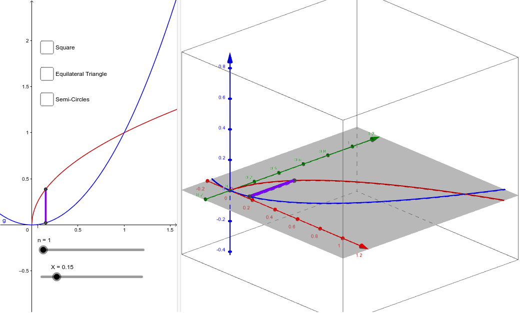
This example provides an interactive visualization for computing volumes of solids using known cross sections. It demonstrates integral calculus concepts, particularly the method of slicing, and connects to solid geometry and continuity. The GeoGebra construction employs the Polygon command to create cross‑section shapes and the Sequence command to generate a series of parallel slices, with objects such as f, g, X, n, A, B, poly1, a, b, c, d, list1, e, h, list3, i, list2 enabling dynamic manipulation. Suitable for high‑school and undergraduate courses in calculus and mathematical modeling.
GeoGebra Commands & Parameters
Polygon((X, f(X), 0), (X, f(X), f(X) - g(X)), (X, g(X), f(X) - g(X)), (X, g(X), 0)) → poly1, a, b, c, dSequence(Polygon[(((k * X)) / n, f(((k * X)) / n), 0), (((k * X)) / n, f(((k * X)) / n), f(((k * X)) / n) - g(((k * X)) / n)), (((k * X)) / n, g(((k * X)) / n), f(((k * X)) / n) - g(((k * X)) / n)), (((k * X)) / n, g(((k * X)) / n), 0)], k, 1, n) → list1Sequence(CircumcircleArc[((k * X / n), f((k * X / n)), 0), ((k * X / n), (f((k * X / n)) + g((k * X / n))) / 2, (f((k * X / n)) - g((k * X / n))) / 2), ((k * X / n), g((k * X / n)), 0)], k, 1, n) → list3Sequence(Polygon[((k * X / n), f((k * X / n)), 0), ((k * X / n), (f((k * X / n)) + g(((k * X)) / n)) / 2, (sqrt(3) * (f((k * X / n)) - g((k * X / n))) / 2)), ((k * X / n), g((k * X / n)), 0)], k, 1, n) → list2