
Visualizing the Tangent of a Function and Its Derivative
Loading the math board and drawing, please wait…
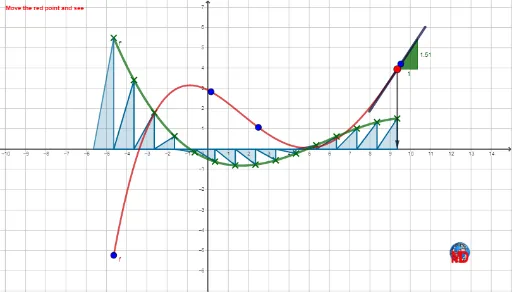
This example dynamically demonstrates the relationship between a function's tangent and its derivative, visually illustrating the geometric meaning of the derivative. Key math concepts include functions, derivatives, tangents, slopes, and limits. Construction highlights involve GeoGebra commands such as Max, Min, Sequence, Point, Intersect, Tangent, Circle, Segment, Slope, Vector, and Polygon to build function graphs, tangents, derivative graphics, and polygons. Suitable for high school students and above, particularly those learning calculus, to understand the intuitive connection and calculation methods between derivatives and tangents.
GeoGebra Commands & Parameters
Max(x(l1)) → bMin(x(l1)) → aSequence((i, f(i)), i, a, b, 1) → l3Point(l3) → FIntersect(If[a ≤ x ≤ b, f'(x)], xAxis) → H, I, JTangent(F, g) → hCircle(F, 2.5) → cIntersect(c, h) → G, KSegment(G, K) → iSequence((i, f'(i)), i, a, b, 1) → l2Sequence(Vector[F, Element[l2, i]], i, 1, Length[l2]) → l4Sequence(Tangent[Element[l3, i], g], i, 1, Length[l3]) → l6Take(l2, 1, x(F) - a + 1) → l5Slope(h) → eSequence(Slope[Element[l6, i]], i, 1, Length[l6]) → l7Sequence((i, 0), i, a, b, 1) → l8Sequence(Polygon[Element[l8, i], Element[l8, i + 1], Element[l2, i + 1]], i, 1, Length[l8]) → l9Vector(F, Element[l8, Length[l5]]) → jTake(l9, 1, x(F) - a) → l10Polygon(Element[l8, 1] - (1, 0), Element[l8, 1], Element[l2, 1]) → t1, k, l, m