
Visualizing Square Numbers by Radha Narve
Loading the math board and drawing, please wait…
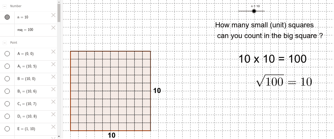
This example dynamically demonstrates the geometric interpretation of square numbers, showing how each natural number's square corresponds to the area of a square. Key math concepts include square numbers, area calculation, number-shape connection, and geometric intuition. Construction highlights involve GeoGebra commands like Polygon, Point, and Segment to form squares, with Slider for dynamic manipulation. Objects include points A, n, nsq, B, and square poly1. Suitable for middle school students and above to learn square numbers, area, and number-shape integration, or as an introductory tool for calculus and linear programming concepts.
GeoGebra Commands & Parameters
Polygon(A, B, 4) → poly1, a, b, c, d, C, DPoint(Circle[A1, n]) → ESegment(A1, E) → ePoint(Circle[A2, n]) → FSegment(A2, F) → fPoint(Circle[A3, n]) → GSegment(A3, G) → gPoint(Circle[A4, n]) → HSegment(A4, H) → hPoint(Circle[A5, n]) → ISegment(A5, I) → iPoint(Circle[A6, n]) → JSegment(A6, J) → jPoint(Circle[A7, n]) → KSegment(A7, K) → kPoint(Circle[A8, n]) → LSegment(A8, L) → lPoint(Circle[A9, n]) → MSegment(A9, M) → mPoint(Circle[A10, n]) → NSegment(A10, N) → pPoint(Circle[A11, n]) → OSegment(A11, O) → qPoint(Circle[A12, n]) → PSegment(A12, P) → rPoint(Circle[A13, n]) → QSegment(A13, Q) → sPoint(Circle[A14, n]) → RSegment(A14, R) → tPoint(Circle[A15, n]) → SSegment(A15, S) → a_1Point(Circle[A16, n]) → TSegment(A16, T) → b_1Point(Circle[B1, n]) → USegment(B1, U) → c_1Point(Circle[B2, n]) → VSegment(B2, V) → d_1Point(Circle[B3, n]) → WSegment(B3, W) → e_1Point(Circle[B4, n]) → ZSegment(B4, Z) → f_1Point(Circle[B5, n]) → A_1Segment(B5, A_1) → g_1Point(Circle[B6, n]) → B_1Segment(B6, B_1) → h_1Point(Circle[B7, n]) → C_1Segment(B7, C_1) → i_1Point(Circle[B8, n]) → D_1Segment(B8, D_1) → j_1Point(Circle[B9, n]) → E_1Segment(B9, E_1) → k_1Point(Circle[B10, n]) → F_1Segment(B10, F_1) → l_1Point(Circle[B11, n]) → G_1Segment(B11, G_1) → m_1Point(Circle[B12, n]) → H_1Segment(B12, H_1) → n_1Point(Circle[B13, n]) → I_1Segment(B13, I_1) → p_1Point(Circle[B14, n]) → J_1Segment(B14, J_1) → q_1Point(Circle[B15, n]) → K_1Segment(B15, K_1) → r_1Point(Circle[B16, n]) → L_1Segment(B16, L_1) → s_1
AI Drawing Prompt Reference
Draw a dynamic visualization showing the geometric meaning of square numbers, where each natural number's square corresponds to the area of a square. Use squares to represent natural numbers, a dynamic slider to control their size, and line segments connecting points and circles to form squares, intuitively demonstrating the connection between numbers and shapes, suitable for learning square numbers, area, and number-shape integration.
The prompt above was compiled from the original drawing commands and is for reference only.