
Visualizing Quadratic Inequalities
Loading the math board and drawing, please wait…
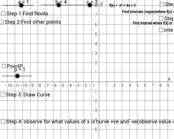
This example is designed for classroom demonstrations on solving quadratic inequalities. It visually represents the solution set of quadratic inequalities through dynamic graphs, illustrating the relationship between the function's graph, its roots, and the inequality. Key mathematical concepts include quadratic functions, solution sets of inequalities, and the connection between graphs and roots. GeoGebra commands used in the construction are Root (to find roots), Function (to plot functions), Extremum (to determine extrema), If (for conditional statements), Segment (to draw line segments), Vector (to create vectors), Midpoint (to find midpoints), and Factor (for factoring expressions). This is suitable for high school mathematics classes to help students grasp the geometric meaning and solving methods of quadratic inequalities.
GeoGebra Commands & Parameters
Root(a * x^(2) + b * x + c) → R_1, R_2Function(a * x^(2) + b * x + c, l_l, l_u) → f_mFunction(a * x^(2) + b * x + c, -70, l_l) → f_lFunction(a * x^(2) + b * x + c, l_u, 100) → fExtremum(a * x^(2) + b * x + c) → TIf(s < 0, 0, If[s ≟ 0, 0, 1]) → colour1If(s < 0, 1, 0) → colour2If(a > 0, 1, If[a ≟ 0, 0, -1]) → sign1Segment(R_2, M_R) → dotted1Vector(M_R, M_RR) → v_1Segment(R_1, M_L) → dotted2Segment(M_IL, M_IR) → jMidpoint(j) → M_imSegment(R_1, M_IL) → dotted3Segment(R_2, M_IR) → dotted4If(a < 0, Simplify[-x + factored2], Simplify[x - factored2]) → factoredexp2If(a^(2) ≟ 0, sgn(b), 1) → v_2signVector(M_L, M_LL) → v_2Factor(f_n) → qIf(sqrt(b^(2) - 4 * a * c) - floor(sqrt(b^(2) - 4 * a * c)) > 0, "Not Factorizable", "Can") → text2ndIf(b^(2) - 4 * a * c < 0, "No Real Roots!", text2nd) → textDetFactor
AI Drawing Prompt Reference
Draw the graph of a quadratic function, showing its vertex and roots, with different colors to indicate the function's values in different intervals. First, plot the function, then mark the roots on the x-axis and draw dashed lines connecting the roots to the vertex. Next, shade the regions above or below the graph based on the sign of the function's coefficients, using different colors to represent the solution set of the inequality. Finally, add text annotations to explain the relationship between the roots, vertex, and the solution set of the inequality.
The prompt above was compiled from the original drawing commands and is for reference only.