
Visualizing Quadratic Equation Solving with Mapping Diagrams
Loading the math board and drawing, please wait…
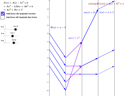
This example demonstrates the solving process of a quadratic equation through mapping diagrams, involving core concepts like quadratic functions, mapping relationships, and coordinate geometry. It is constructed using GeoGebra commands and objects such as Point, Vector, Textfield, and Sequence, making it suitable for high school mathematics education to help students understand the connection between functions and equations.
GeoGebra Commands & Parameters
Point(yAxis) → A_xVector(A_x, B) → uVector(B, C) → vTextfield(m) → inputBox1Textfield(s) → inputBoxfSequence(Vector[(6, m(q(R(i)))), (8, s(m(q(R(i)))))], i, 1, 5) → QuadgvlistSequence(Vector[(4, q(R(i))), (6, m(q(R(i))))], i, 1, 5) → QuadmvlistSequence(Vector[(0, i), (2, R(i))], i, 1, 5) → QuadRvlistSequence(Vector[(2, R(i)), (4, q(R(i)))], i, 1, 5) → QuadqvlistPoint(i) → KVector(K, s_{inv}D) → wVector(s_{inv}D, m_{invSinvD}) → zVector(m_{invSinvD}, q_{inv+}) → dVector(m_{invSinvD}, q_{inv-}) → fVector(q_{inv+}, I) → h_1Vector(q_{inv-}, J) → jSequence(Vector[(0, i), (2, m(i))], i, -2, 2) → LinmvlistSequence(Vector[(2, m(i)), (4, s(m(i)))], i, -2, 2) → LingvlistTextfield(h) → inputBox2Textfield(k) → inputBox3Textfield(A) → inputBox4
AI Drawing Prompt Reference
Create a mapping diagram to visualize the solving process of a quadratic equation. Include a horizontal axis and a curve representing a quadratic function. Mark several points on the curve and use vectors to show the relationship between these points and their function values. Add input boxes for users to enter parameters, and use vectors to illustrate how these parameters affect the mapping diagram. Finally, connect key points with vectors to demonstrate the mapping relationship between function values and parameters, making the solving process of the quadratic equation clear and intuitive.
The prompt above was compiled from the original drawing commands and is for reference only.