
Visualizing Linear Transformations: Vectors and Polygons Under Matrix Action
Loading the math board and drawing, please wait…
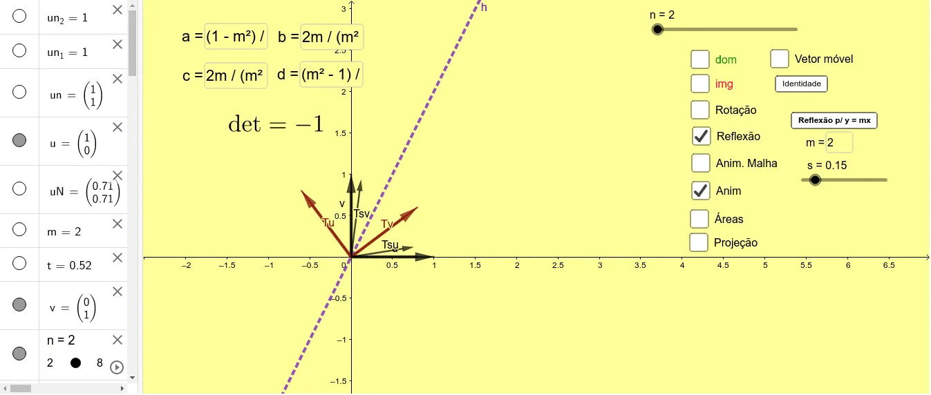
① This interactive GeoGebra example demonstrates how linear transformations act on vectors and polygons in the plane, allowing users to adjust parameters and observe stretching, rotation, or shearing effects in real time. ② Core mathematical concepts include linear transformations, matrix multiplication, vector mapping, changes in basis vectors, and effects on area and orientation, forming foundational linear algebra knowledge. ③ Construction highlights: uses GeoGebra commands such as Vector to create vectors, Sequence for point generation, Polygon to build shapes, and Length for measurements; Textfield and InputBox provide parameter inputs, while a button triggers the transformation; objects include multiple vectors (u, v, w and their images Tu, Tv, Tw) and transformed polygons (Tsu, Tsv), with sliders and input boxes dynamically controlling matrix elements. ④ Suitable for high school to early university students, this example aids in understanding the geometric meaning of matrix transformations in linear algebra courses, and serves as an effective classroom demonstration tool for teachers to bridge algebraic and geometric intuition.
GeoGebra Commands & Parameters
Vector((0, 1)) → vVector(((a * x(u)) + (b * y(u)), (c * x(u)) + (d * y(u)))) → TuVector(((a * x(v)) + (b * y(v)), (c * x(v)) + (d * y(v)))) → TvSequence(Sequence[Vector[Point[(0, 0), Vector[(i * u) + (j * v)]], Point[(0, 0), Vector[(i * u) + (j * v)]] + v], i, (-n), n], j, (-n), n) → l2Sequence(Sequence[Vector[Point[(0, 0), Vector[(i * u) + (j * v)]], Point[(0, 0), Vector[(i * u) + (j * v)]] + u], i, (-n), n], j, (-n), n) → l1Sequence(Sequence[Vector[Point[(0, 0), Vector[(i * Tu) + (j * Tv)]], Point[(0, 0), Vector[(i * Tu) + (j * Tv)]] + Tv], i, (-n), n], j, (-n), n) → l3Sequence(Sequence[Vector[Point[(0, 0), Vector[(i * Tu) + (j * Tv)]], Point[(0, 0), Vector[(i * Tu) + (j * Tv)]] + Tu], i, (-n), n], j, (-n), n) → l4Textfield(a) → InputBox1Textfield(b) → InputBox2Textfield(c) → InputBox3Textfield(d) → InputBox4Textfield(t) → InputBox5Textfield(m) → InputBox6Vector((0, 0), A) → wVector(((a * x(w)) + (b * y(w)), (c * x(w)) + (d * y(w)))) → TwVector((((1 - s + (s * a)) * x(u)) + ((s * b) * y(u)), ((s * c) * x(u)) + ((1 - s + (s * d)) * y(u)))) → TsuVector((((1 - s + (s * a)) * x(v)) + ((s * b) * y(v)), ((s * c) * x(v)) + ((1 - s + (s * d)) * y(v)))) → TsvSequence(Sequence[Vector[Point[(0, 0), Vector[(i * Tsu) + (j * Tsv)]], Point[(0, 0), Vector[(i * Tsu) + (j * Tsv)]] + Tsv], i, (-n), n], j, (-n), n) → l5Sequence(Sequence[Vector[Point[(0, 0), Vector[(i * Tsu) + (j * Tsv)]], Point[(0, 0), Vector[(i * Tsu) + (j * Tsv)]] + Tsu], i, (-n), n], j, (-n), n) → l6Polygon(E, B, D, C) → q1, e_1, b_1, d_1, c_1Polygon(E, F, H, G) → q2, e_2, f_1, h_1, g_1Textfield(un_1) → InputBox7Textfield(un_2) → InputBox8Length(uN) → p
AI Drawing Prompt Reference
Create a 2D plane illustrating a linear transformation acting on vectors and polygons. Draw two basis vectors from the origin and their images under the matrix, using distinct colors. Generate a grid of lines formed by integer combinations of the basis vectors, and also show the transformed grid. Include a draggable point and its transformed image, connected by arrows. Construct two polygons, one original and one transformed, with vertices labeled. Provide input boxes and sliders to adjust matrix entries, transformation parameters, and grid extent, updating the visualization dynamically.
The prompt above was compiled from the original drawing commands and is for reference only.