Visualizing Linear Equation ax+by=c

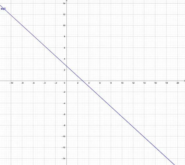
This example dynamically demonstrates the graph of linear equation ax+by=c, showing how the position and slope of the line change with variations in coefficients a, b, and c. Key math concepts include linear equations, coordinate geometry, line slope and intercept, and matrix operations. GeoGebra commands used are objects a, b, c, eq1 for defining parameters and equations, with sliders for dynamic adjustments. Suitable for high school students and teachers to understand the geometric meaning of linear equations and parameter effects, also showcasing matrix applications.