Cramer's Rule for Solving Linear Equations

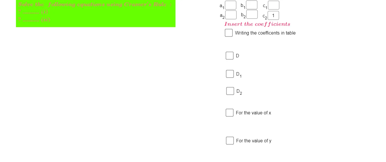
① This activity uses Cramer's Rule to demonstrate how to solve linear equation systems using matrices. ② It covers determinants, matrix representation of linear equations, the step‑by‑step computation of Cramer's Rule, and dynamic adjustment of parameter variables. ③ In GeoGebra, Textfield and InputBox controls create adjustable coefficients; matrix objects a, b, c, etc., build the coefficient matrix and constant vector; eq1, eq2, and related objects display the real‑time calculation process after formula substitution. ④ Designed for high‑school or university freshman linear algebra courses, as well as for dynamic demonstrations in teaching or self‑study.