Visualizing Epsilon-Delta Definition of Limits

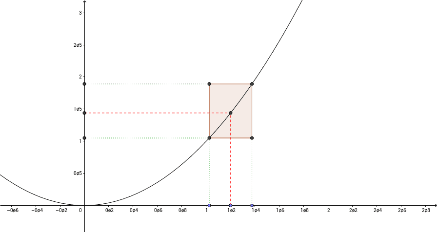
This GeoGebra example offers an intuitive, notation-first approach to the epsilon-delta definition of limits. It demonstrates the geometric relationship between a delta neighborhood around input a and an epsilon neighborhood around the limit L, showing how function values f(x) stay within the target band when x is sufficiently close to a. Core mathematical concepts include limits, continuity, neighborhoods, and the formal inequalities |x − a| < δ and |f(x) − L| < ε. The construction relies on GeoGebra commands Point, Distance, OrthogonalLine, Intersect, Polygon, and Segment, utilizing objects such as f, G, A, distanceAG, a, B, b, C, D, c, d, E, F, poly1, c_1, e, d_1, f_1, H, I, g, h, i, j, k, J, l, K, m, n, and TextAG to create dynamic epsilon-delta rectangles, perpendicular lines, and intersection points. It is ideal for pre-calculus learners and first-year university calculus or analysis courses seeking a visual foundation before formal symbolic study.