
Visualizing Complex Roots of a Quadratic Equation
Loading the math board and drawing, please wait…
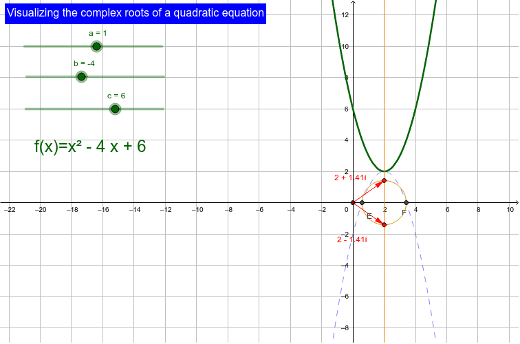
This example demonstrates how to visualize complex roots of a quadratic equation using GeoGebra, illustrating the relationship between complex roots and the graph. Core math concepts include quadratic equations, complex numbers, discriminant, function graphs. Key GeoGebra commands/objects used are Intersect, OrthogonalLine, Mirror, Circle, ComplexRoot, and Vector as derived from the construction summary. Suitable for high school mathematics education to help students understand the geometric meaning and properties of complex roots.
GeoGebra Commands & Parameters
Intersect(f, xAxis) → A, BOrthogonalLine(P, xAxis) → dIntersect(f, d) → CMirror(f, C) → f_1Intersect(f_1, xAxis) → E, FCircle(P, F) → eIntersect(xAxis, yAxis) → GIntersect(e, d, 2) → HComplexRoot(f) → z_1, z_2Vector(G, z_1) → uVector(G, z_2) → v
AI Drawing Prompt Reference
Draw the graph of a quadratic function that intersects the horizontal axis at two points. Choose a point on the graph and draw a vertical line through it perpendicular to the axis, intersecting the graph again at another point. Reflect the entire graph across this second point to obtain a new curve, which crosses the horizontal axis at two points. Using the original point on the graph as the center, draw a circle passing through one of the new curve's axis intersections; this circle meets the vertical line at a point. Finally, from the origin, draw two vectors pointing to the complex roots in the complex plane, which correspond to the new curve's axis intersections.
The prompt above was compiled from the original drawing commands and is for reference only.