
Visualizing Complex Numbers & Polynomials
Loading the math board and drawing, please wait…
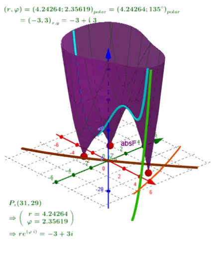
① This example demonstrates the graphical representation of complex polynomials and a polar‑based root‑finding animation on the complex plane. ② Core mathematical concepts include algebraic and polar forms of complex numbers, polynomials with rational and complex coefficients, distribution of zeros, and the real/imaginary surface of the function. ③ Construction highlights: GeoGebra commands Rotate, Surface, CurveCartesian, Locus, Sequence build dynamic surfaces and loci; interactive objects Textfield, InputBox, Button enable parameter entry and step control; objects a₄, a₃, a₂, a₁, a₀, Z₀…Z₄, ROOTS, KRoots store coefficients, variables, and roots; auxiliary quantities Length, φ, incφ, ktan, ctan drive the polar iteration. ④ Suitable for high‑school pre‑calculus through introductory university complex analysis, and for self‑study of visualizing complex polynomial zeros.
GeoGebra Commands & Parameters
Rotate(g, π / 2, xAxis) → pSurface(u, v, abs(f_{R}(u, v) + (ί * f_{I}(u, v))), u, -10, 10, v, -10, 10) → absFCurveCartesian(t, 0, abs(f_{R}(t, 0) + (ί * f_{I}(t, 0))), t, -10, 10) → f_1Locus(P_{z}, φ) → Z_{r,φ}Locus(P_{z}, r) → Z_rTextfield(KRoots) → InputBox1Length(CKRoots) → n_{CKR}Sequence({abs(Element[R, j]), ctan(x(Element[R, j]), y(Element[R, j]))}, j, 1, Length[R]) → Rphi
AI Drawing Prompt Reference
Visualize complex polynomials on the complex plane, showing algebraic and polar forms, with dynamic surfaces and loci for zero distribution and real/imaginary parts. Draw polynomial curves, create rotating trajectories and polar iteration animations, control parameters with sliders, and use text fields and buttons for interactive input and step control.
The prompt above was compiled from the original drawing commands and is for reference only.