
Visualizing Complex Differential with Mapping Diagram
Loading the math board and drawing, please wait…
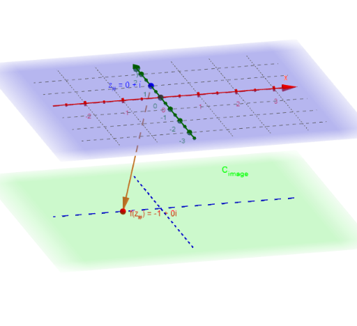
This example uses a mapping diagram to visualize complex differential. It involves the derivative of complex functions and dynamically adjusts parameters to observe changes in the function's graph. Main commands used include Sequence, CurveCartesian, Vector, Textfield, Intersect, and Derivative. Suitable for complex analysis studies in university mathematics.
GeoGebra Commands & Parameters
Sequence((r * (cos(t) + (sin(t) * ί))), t, -3.141592653589793, 3.141592653589793, 0.5235987755982988) → z_*Sequence((x(Element[fz_*, k]), y(Element[fz_*, k]), height_{image}), k, 1, 12) → fpoint_*Sequence(Vector[Element[z_*, j], Element[fpoint_*, j]], j, 1, 12) → fvec_*CurveCartesian((r * cos(t)), (r * sin(t)), height_{image}, t, 0, 6.283185307179586) → dVector(z_#, f_{(z#).}) → wCurveCartesian(t, 0, height_{image}, t, -5, 5) → XhCurveCartesian(0, t, height_{image}, t, -5, 5) → YhTextfield(z_*) → inputBox3Vector(z_#, z_1) → uIntersect(xAxis, yAxis) → AVector(A, Δz) → vCurveCartesian((r * cos(t)), (r * sin(t)), t, t_a, t_b) → γTextfield(t_a) → inputBox4Textfield(t_b) → inputBox5Sequence(t_a + (k / m * (t_b - t_a)), k, 0, m) → t_*Derivative(f, z) → dfVector(A, Δw) → hVector(f_{(z#).}, f_{z1}) → gVector(z_1, f_{z1}) → iTextfield(F) → InputBox1Vector(f_{(z#).}, Diff_#) → l