
Visualize the area of a circle
Loading the math board and drawing, please wait…
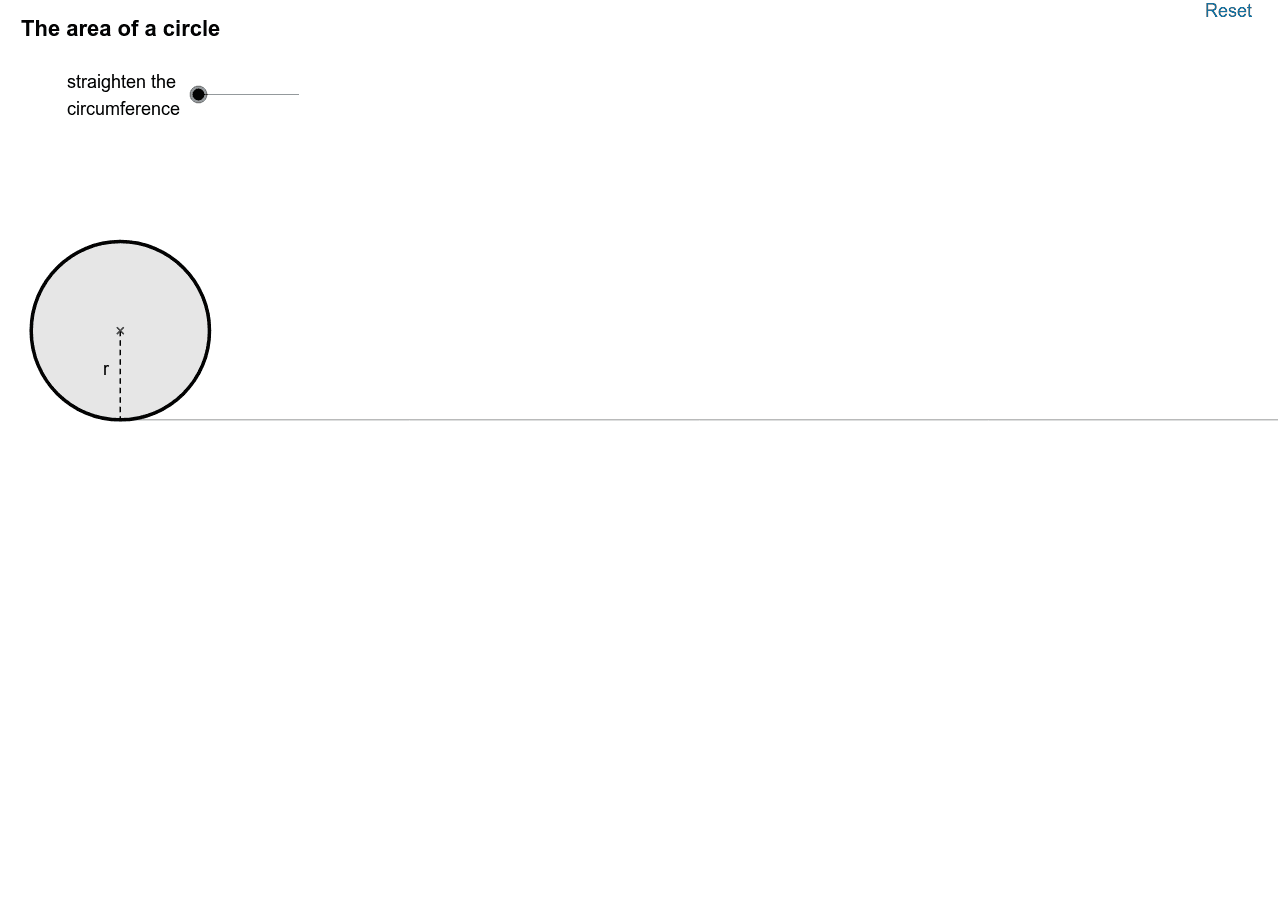
This example demonstrates the concept of the area of a circle using dynamic geometry. Key mathematical concepts include area calculation, geometric construction, and parametric representation. Construction involves GeoGebra commands such as Circle, Sector, and Arc. Suitable for middle school or high school students learning geometry and mathematical formulas.
GeoGebra Commands & Parameters
Segment(E, (x(E) + 2, y(E))) → aPoint(a) → FMin(x(F) - x(E), 1) → kPoint(yAxis) → OSequence(If[k < 1, (x(O) + ((l * sin((i * φ))) * cos((i * φ)) / sin(φ)), y(O) + ((l * sin((i * φ))) * sin((i * φ)) / sin(φ))), (x(O) + (l * i), y(O))], i, 0, (2 * n)) → list2Sequence((x(O) + sin((i * θ)), y(O) + 1 - cos((i * θ))), i, 0, (2 * n)) → list1Max(x(F) - x(E) - 1, 0) → k'Rotate((x(O) + 0, y(O) + 1), ((-k) * θ / 2), O) → ARotate(O, ((-k) * θ / 2), O) → O'Rotate(Element[list1, 1], ((-k) * θ / 2), O) → BSector(Rotate[Circle[(x(O) + 0, y(O) + 1), O], ((-k) * θ / 2), O], Rotate[O, ((-k) * θ / 2), O], Rotate[Element[list1, 1], ((-k) * θ / 2), O]) → cRotate((x(O) + 0, y(O) + 1), ((-k) * θ / 2), O) → CRotate(O, ((-k) * θ / 2), O) → O'_1Rotate(Element[list1, 1], ((-k) * θ / 2), O) → DArc(Rotate[Circle[(x(O) + 0, y(O) + 1), O], ((-k) * θ / 2), O], O'_1, D) → dCurveCartesian(t - sin(t), 1 - cos(t), t, 0, 6.28319) → bCircle((0, 1), 1) → hRay((0, 0), (1, 0)) → iPoint(Segment[(0, 1), (6.28319, 1)]) → HSegment(H, (x(H), 0)) → jMidpoint(j) → IMidpoint(a) → JCircle(L, 1 / (1 - m)) → pCircle((0, 0), 1 / (1 - m)) → qIntersect(p, q, 1) → MIntersect(p, q, 2) → NCircle((0, 1), 1) → c_1Segment((0, 0), (6.283185307179586, 0)) → eSegment(G, (x(G), y(G) - 1)) → rSequence(Sector[Rotate[Translate[Circle[(x(O) + 0, y(O) + 1), Element[list1, i]], Vector[Element[list1, i], Element[list2, i]]], (((-((2 * i) - 1)) * k) * θ / 2), Element[list2, i]], Rotate[Translate[Element[list1, i], Vector[Element[list1, i], Element[list2, i]]], (((-((2 * i) - 1)) * k) * θ / 2), Element[list2, i]], Rotate[Translate[Element[list1, i + 1], Vector[Element[list1, i], Element[list2, i]]], (((-((2 * i) - 1)) * k) * θ / 2), Element[list2, i]]], i, 1, n) → list3Sequence(Sector[Rotate[Rotate[Translate[Circle[(x(O) + 0, y(O) + 1), Element[list1, i]], Vector[Element[list1, i], Element[list2, i]]], (((-((2 * i) - 1)) * k) * θ / 2), Element[list2, i]], (180° * k'), (x(O) + (n * l) - sin(θ / 2) / 2, y(O) + cos(θ / 2) / 2)], Rotate[Rotate[Translate[Element[list1, i], Vector[Element[list1, i], Element[list2, i]]], (((-((2 * i) - 1)) * k) * θ / 2), Element[list2, i]], (180° * k'), (x(O) + (n * l) - sin(θ / 2) / 2, y(O) + cos(θ / 2) / 2)], Rotate[Rotate[Translate[Element[list1, i + 1], Vector[Element[list1, i], Element[list2, i]]], (((-((2 * i) - 1)) * k) * θ / 2), Element[list2, i]], (180° * k'), (x(O) + (n * l) - sin(θ / 2) / 2, y(O) + cos(θ / 2) / 2)]], i, n + 1, (2 * n)) → list4CircleArc((0, 1 / (1 - m)), O, L) → s
AI Drawing Prompt Reference
Draw a dynamic visualization of the area of a circle: on the left, a circle with radius 1 centered above the origin, divided into equal sectors that are translated and rotated to gradually form an approximate rectangle on the right; include a horizontal line representing the unfolded circumference, a cycloid curve as a reference, and a draggable point to control the number of divisions, showing how the circle's area equals πr².
The prompt above was compiled from the original drawing commands and is for reference only.