
Using Normal Distributions for Experiment Analysis (Practice)
Loading the math board and drawing, please wait…
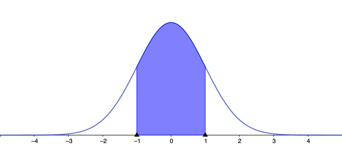
This example demonstrates how to model experimental variability using a normal (Gaussian) distribution and how the distribution’s shape connects to probability statements used in experiment analysis. The key mathematical ideas include the normal distribution model, parameters such as mean and variance (standard deviation), the probability density function (and related cumulative probability reasoning), and how changing parameters alters the graph to support interpretation of results. Construction typically centers on GeoGebra graphing: defining the normal distribution as a function of x with adjustable parameters, plotting the density curve, and optionally highlighting probability between intervals by shading or evaluating regions. Suitable for high school onward through early undergraduate probability & statistics, as well as data modeling and classroom demonstration.
AI Drawing Prompt Reference
In a single coordinate plane, draw and illustrate a normal (Gaussian) probability density curve: use the horizontal axis for x values and the vertical axis for probability density. Create a curve defined by a normal model whose parameters can be adjusted, with controls for the mean and the standard deviation so the user can see how shifting the mean and changing the spread reshape the graph. Optionally, for an interval, indicate its endpoints and visually emphasize the area under the curve between them (or provide an interval-probability interpretation) to connect the density shape to probability statements used in experiment analysis.
The prompt above was compiled from the original drawing commands and is for reference only.