
Unit Circle with sin2x Dynamic Visualization
Loading the math board and drawing, please wait…
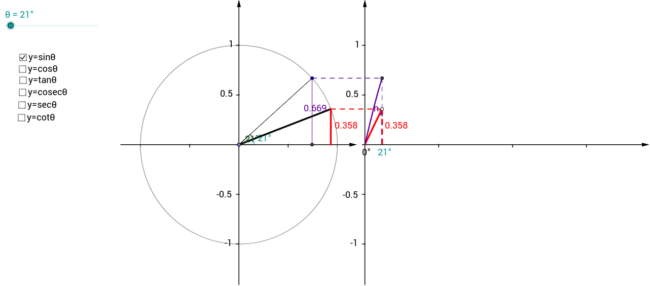
① This example visually demonstrates the sine function sin(2x) on the unit circle, connecting the angle's rotation to the function's value as a projection. ② Core mathematical concepts include the unit circle, trigonometric functions (sine), radian measure, function graphing, and the double-angle relationship. ③ Construction uses GeoGebra commands: Point, Rotate, Angle, Function, Segment, Circle, Vector, and Sequence, creating rotating points, angle sliders, function curves, vectors, and sequences, with text labels for key values. ④ Ideal for high school or introductory college students studying trigonometry and the unit circle, and for teachers demonstrating the geometric intuition behind the double-angle formula.
GeoGebra Commands & Parameters
Point(Ray[(0, 0), (-1, 0)]) → BRotate(A, θ, B) → PRotate(A, θ, B) → A'Angle(A, B, A') → αRotate(A, θ, B) → A'_1Angle(A, B, A'_1) → βFunction(sin((120° * x)), 0, x(Q)) → fSegment(Q, (x(Q), 0)) → eCircle(B, A) → cSegment(B, P) → aVector((x(B), y(Corner[1])), (x(B), y(Corner[4]))) → uVector((0, y(Corner[1])), (0, y(Corner[4]))) → wVector((0, 0), (x(Corner[2]), 0)) → zSequence(Segment[((0.75 * i), 0), ((0.75 * i), -0.025)], i, 1, 4) → list1Segment(P, (x(P), 0)) → bVector(B - (1.2, 0), B + (1.2, 0)) → vSequence(Segment[(0, (0.5 * i) - 1), (-0.025, (0.5 * i) - 1)], i, 0, 4) → list2Sequence(Segment[(x(B), (0.5 * i) - 1), (x(B) - 0.025, (0.5 * i) - 1)], i, 0, 4) → list3Segment(P, Q) → dSequence(Segment[B + ((0.5 * i) - 1, 0), B + ((0.5 * i) - 1, -0.025)], i, 0, 4) → list4Point(Ray[(0, 0), (-1, 0)]) → B_1Rotate(A_1, θ, B_1) → P_1Rotate(A_1, θ, B_1) → A'_2Rotate(A_1, θ, B_1) → A'_3Circle(B_1, A_1) → c_1Segment(B_1, P_1) → a_1Point(b) → CPoint(list3) → DSegment(C, D) → hFunction(cos((120° * x)), 0, x(Q)) → pSegment(E, (x(E), 0)) → iSegment(D, (x(P), 0)) → jPoint(c) → GSegment(C, H) → lSegment(H, G) → mFunction(tan((120° * x)), 0, (θ / ((360 * γ)) * 3)) → qSegment(I, (x(I), 0)) → nSegment(H, I) → rSegment(C, J) → sSegment(C, K) → tSegment(K, D) → b_1Segment(D, J) → d_1Function(csc((120° * x)), 0, x(Q)) → f_1Segment(J, L) → e_1Segment(L, (x(L), 0)) → g_1Function(sec((120° * x)), 0, (θ / ((360 * γ)) * 3)) → p_1Segment(M, (x(M), 0)) → i_1Segment(C, K) → j_1Point(list3) → NSegment(O, N) → l_1Segment(C, O) → m_1Function(cot((120° * x)), 0, x(Q)) → q_1Segment(R, (x(R), 0)) → n_1Segment(C, J) → r_1Rotate(A, (2 * θ), B) → A'_4Segment(A'_4, D) → s_1Angle(C, D, A'_4) → δSegment(A'_4, S) → f_2Segment(A'_4, T) → g_2Segment(T, (x(T), 0)) → h_2
AI Drawing Prompt Reference
Draw a unit circle centered at the origin with radius 1. Place a moving point on the circle, controlled by an angle slider. Draw a radius segment from the center to this point. Outside the circle, set up a coordinate system with the horizontal axis for angle and vertical axis for function values. Plot the sine function sin(2x) from 0 to the current angle, and project the point's vertical coordinate onto this curve using a perpendicular segment. Label the angle on the circle. Additionally, plot cosine, tangent, cosecant, and secant curves in different colors or line styles. Add tick marks below the circle for key angle values.
The prompt above was compiled from the original drawing commands and is for reference only.