
Understanding Sample Distributions
Loading the math board and drawing, please wait…
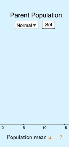
This example demonstrates how to dynamically visualize the generation and variation of sample distributions using GeoGebra. Core math concepts include sample distributions, normal distributions, skewed distributions, and data statistics. Key GeoGebra commands and objects used are Sequence, If, Max, Min, Histogram, LaTeX, along with elements like bins, skewed/normal data types, and sliders for control. Suitable for high school mathematics and statistics education to help students intuitively grasp the characteristics of sample distributions and statistical principles.
GeoGebra Commands & Parameters
Sequence(round(InverseChiSquared[3, RandomUniform[0, 1]]), i, 0, 100) → skeweddataSequence(round(RandomNormal[8, 3]), i, 0, 100) → normaldataIf(normal ≟ true, normaldata, skewed ≟ true, skeweddata) → dataMax(data) → xmaxMin(data) → xminSequence(xmin + (i * bins), i, 0, ceil(range / bins)) → sequenceHistogram(sequence, data) → parenthistogramSequence(mean[First[Shuffle[data], slider1]], i, 1, trials) → sampledistributionHistogram(sequence, sampledistribution) → samplehistogramLaTeX(normaldata, true, true) → text1
AI Drawing Prompt Reference
Create a histogram showing both normal and skewed distributions of sample data, controlled by sliders for sample size and distribution type. First, generate 100 skewed data points, then 100 normal data points. Use the slider to switch between displaying data from the normal or skewed distribution. Calculate the maximum and minimum values of the data, set the histogram bins, and draw the histogram. Also, display the statistical description of the normal distribution data.
The prompt above was compiled from the original drawing commands and is for reference only.