
Two-way Tables and Conditional Probability Dynamic Simulation
Loading the math board and drawing, please wait…
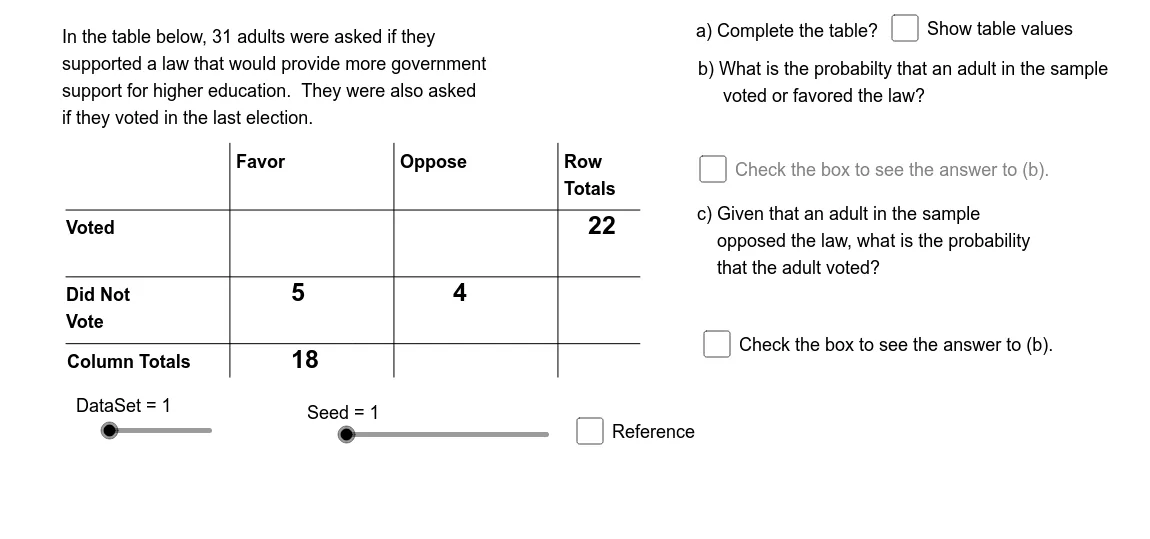
This GeoGebra example demonstrates the construction of two-way tables and the calculation of conditional probabilities through dynamic random simulation. It generates a dataset with two categorical variables, displays the frequency counts in a contingency table, and computes joint, marginal, and conditional probabilities along with expected values. The core mathematical concepts include conditional probability, joint probability, marginal probability, expected value, and random simulation. The construction uses commands such as Random, Element, Min, Mod, Segment, If, Append, and objects like Seed, DataSet, Pr12Sq, Tb11, and sliders (SlNm1, SlNm2) to control sample size or parameters. It is suitable for high school or introductory college statistics courses to illustrate probability concepts, contingency tables, and the law of large numbers through interactive exploration.
GeoGebra Commands & Parameters
Element(Pr12Sq, DataSet) → Pr12Element(Pr22Sq, DataSet) → Pr22Element(Pr21Sq, DataSet) → Pr21Element(Pr11Sq, DataSet) → Pr11Min({Pr11, Pr12, Pr21, Pr22}) → PrMinMod(SlNm2, 2) → BOpElement(DDSq, DataSet) → DD0Element(RL1Sq, DataSet) → RL1Element(RL2Sq, DataSet) → RL2Element(CL1Sq, DataSet) → CL1Element(CL2Sq, DataSet) → CL2Segment((TbLf, TbTp - TbCH), (TbLf + (3.5 * TbCW), TbTp - TbCH)) → htpSegment((TbLf, TbTp - (2 * TbCH)), (TbLf + (3.5 * TbCW), TbTp - (2 * TbCH))) → hmdSegment((TbLf, TbTp - (3 * TbCH)), (TbLf + (3.5 * TbCW), TbTp - (3 * TbCH))) → hbmSegment((TbCW, TbTp), (TbCW, TbTp - (3.5 * TbCH))) → vlfSegment(((2 * TbCW), TbTp), ((2 * TbCW), TbTp - (3.5 * TbCH))) → vmdSegment(((3 * TbCW), TbTp), ((3 * TbCW), TbTp - (3.5 * TbCH))) → vrgElement(IndSq, DataSet) → IndElement(Rw1OpSq, DataSet) → Op1Element(Rw2OpSq, DataSet) → Op2Element(Cl1OpSq, DataSet) → Op3Element(Cl2OpSq, DataSet) → Op4If(OpBNm1 > 2, OpBNm2, OpBNm2 + 2) → OpBNm3Element(OpSq, OpANm1) → OpA1Element(OpSq, OpANm2 + 2) → OpA2Element(OpSq, OpBNm1) → OpC1Element(OpSq, OpBNm3) → OpC2Element(TbRCSq, OpANm1) → TbRwElement(TbRCSq, OpBNm1) → CndRCElement(CndRC, OpBNm2) → BNumElement(RCTtSq, OpBNm1) → BDnmAppend(TbRw, Element[Element[TbRCSq, OpANm3], OpANm2]) → OpASqElement(OpASq, 1) → ANm1Element(OpASq, 2) → ANm2Element(OpASq, 3) → ANm3If(DataSet ≟ 1, "an", "a") → IARandom(1, 2) → baRandom(1, 2) → bbRandom(1, 2) → bcRandom(1, 2) → bdElement(IndSq_1, DataSet) → Ind_1Element(Rw1OpSq_1, DataSet) → Op1_1Element(Rw2OpSq_1, DataSet) → Op2_1Element(Cl1OpSq_1, DataSet) → Op3_1Element(Cl2OpSq_1, DataSet) → Op4_1Element(OpSq_1, OpANm1_1) → OpA1_1Element(OpSq_1, OpANm2_1 + 2) → OpA2_1If(DataSet ≟ 1, "an", "a") → IA_1
AI Drawing Prompt Reference
Create a dynamic chart showing a random dataset with two categorical variables, displaying frequency counts in a table and calculating joint, marginal, and conditional probabilities. Include sliders to control parameters, generate data through random simulation, and draw lines for the table and probability bars to visually illustrate probability concepts and expected values.
The prompt above was compiled from the original drawing commands and is for reference only.