
Two Poisson Distributions: Page 21
Loading the math board and drawing, please wait…
In collections
Pearson Maths A level Further Statistics 1
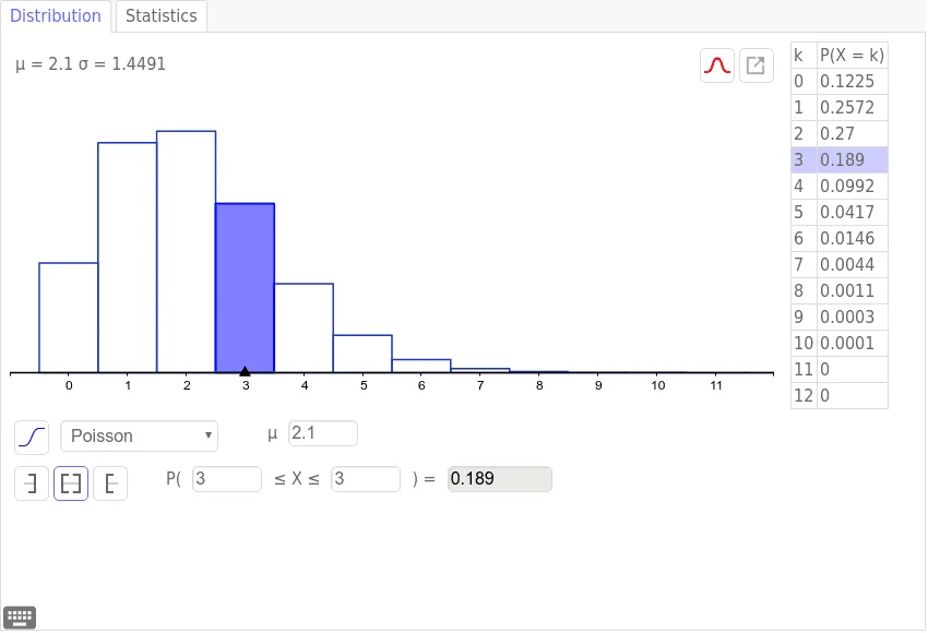
①This example visually compares the probability mass functions of two Poisson distributions with different parameters (λ) using bar charts, highlighting differences in shape and the range of random variable values. ②Core mathematical concepts include the Poisson distribution, a discrete probability distribution modeling the number of events in a fixed interval, with parameter λ affecting both mean and variance. ③Construction details: The GeoGebra commands used include BarChart for plotting bars, Sequence for generating value sequences, Take, Min, and Max for extracting data ranges, Point for marking key coordinates, RotateText for rotating text labels, and lists list1 through list6 storing distribution values and auxiliary data; objects A, B, a, b control parameters or coordinates. ④This resource suits high school to undergraduate probability and statistics courses, useful for demonstrating how the Poisson distribution shifts and widens as λ changes, and as an interactive tool for exploring discrete distributions and parameter sensitivity.
GeoGebra Commands & Parameters
RotateText("y", 0) → text3RotateText("x", 0) → text4Sequence(Segment[(-100, i), (100, i)], i, -50, 50, 0.1) → list1Sequence(Segment[(-100, i), (100, i)], i, -50, 50, 0.5) → list2Sequence(Segment[(i, -100), (i, 100)], i, -50, 50, 0.1) → list3Sequence(Segment[(i, -100), (i, 100)], i, -50, 50, 0.5) → list4Point(xAxis) → APoint(xAxis) → BBarChart({0, 1, 2, 3, 4, 5, 6, 7, 8, 9, 10, 11, 12}, {0.013841287201, 0.071183762748, 0.167790297906, 0.23970042558, 0.231139696095, 0.158495791608, 0.079247895804, 0.029111471928, 0.00779771569500003, 0.00148527918, 0.000190964466000001, 0.0000148803480000001, 5.31440999999999E-7}, 1) → aTake({0.013841287201, 0.071183762748, 0.167790297906, 0.23970042558, 0.231139696095, 0.158495791608, 0.079247895804, 0.029111471928, 0.00779771569500003, 0.00148527918, 0.000190964466000001, 0.0000148803480000001, 5.31440999999999E-7}, x(A) + 1.5, x(B) + 1.5) → list5Take({0, 1, 2, 3, 4, 5, 6, 7, 8, 9, 10, 11, 12}, x(A) + 1.5, x(B) + 1.5) → list6BarChart(list6, list5, 1) → bSequence(12, 12, 0, InversePoisson[2.1, 0.999999]) →Min(x(Point[xAxis]) + 1.5, x(Point[xAxis]) + 1.5) →Max(x(Point[xAxis]) + 1.5, x(Point[xAxis]) + 1.5) →
AI Drawing Prompt Reference
Draw bar charts to compare the probability mass functions of two Poisson distributions with different parameters λ, highlighting differences in shape and the range of random variable values. Include horizontal line grids, labeled axes, and plot two distributions with λ=2.1 and λ=2.1 in different colors, with bar widths of 1.5 units and shifted 1.5 units along the x-axis.
The prompt above was compiled from the original drawing commands and is for reference only.