Truncated Icosahedron: Average Vertex Distance vs Truncation Parameter and Extre

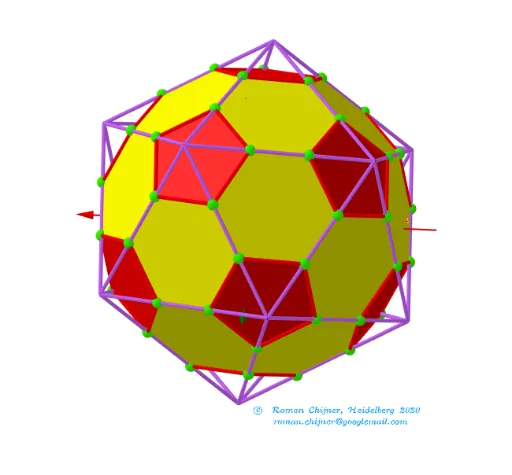
①This example demonstrates how the average distance between vertices of a truncated icosahedron (an Archimedean solid) changes with the truncation parameter, and shows the extreme distribution of this average. ②Core mathematical concepts include solid geometry of polyhedron truncation, statistical averaging of inter-vertex distances, optimization problems, and function graphs with parameter-dependent extrema. ③Construction highlights: using GeoGebra commands such as Join, Unique, Length, Sum, Sphere, Ray, Zip, UnicodeToLetter, and TableText to build vertex sets and distance computations; a slider controls the truncation parameter t, dynamically updating vertex list lP' and distance list lVV, and plotting the average distance function; buttons and text objects display results, involving objects like polyhedron vertices, spheres, rays, and table text. ④Suitable for high school to university mathematics teaching, for exploring solid geometry, optimization, and parametric modeling, as well as for math labs or competition enrichment.