
Torus Loxodrome and Related Constructions
Loading the math board and drawing, please wait…
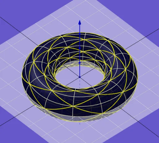
① This example demonstrates drawing a loxodrome (a curve making a constant angle with the meridians) on a torus, along with various related geometric objects such as circles, segments, polygons, and surfaces. ② Core mathematical concepts include parametric equations of a torus, space curves (CurveCartesian), surfaces (Surface), geometric transformations (Mirror), sequences (Sequence), and the use of least common multiple (LCM) to create periodic patterns. ③ Construction highlights: GeoGebra commands such as Point, Segment, Circle, CircleArc, Midpoint, Intersect, Line, Mirror, LCM, Sequence, Polygon, Surface, CurveCartesian, OrthogonalLine, Zip, OrthogonalPlane, KeepIf, Unique are used to build the torus, loxodrome, auxiliary circles, tangents, normals, and repeated structures generated by sequences; objects include g_y, J, I, j, F, R, mTr, r, rTr, e, g_x, o, f, K, f_1, A, c, B, C, g_d, eTR, etc. ④ Suitable for high school to university-level mathematics teaching, for exploring 3D geometry, parametric curves and surfaces, transformations and sequences, and as an example for mathematical modeling or computer-aided geometric design.
GeoGebra Commands & Parameters
Point(g_y) → JPoint(g_y) → ISegment(I, J) → jPoint(j) → FCircle(mTr, rTr) → ePoint(g_x) → oCircle(o, F) → fPoint(f) → KCircleArc(o, F, K) → f_1Midpoint(o, mTr) → ACircle(A, mTr) → cIntersect(e, c) → B, C, ,Line(o, C) → g_dMirror(eTR, xAxis) → eTR'_1Mirror(eTR, g_x) → eTR'Mirror(eTR', xAxis) → eTR''LCM(n', m') → kgvAnzSequence(k, k, (-kgvAnz), kgvAnz) → ListkgvMirror(g_d, g_x) → g'_dIntersect(g'_d, gl1) → EPolygon(eTR, eTR', eTR'', eTR'_1) → v1, h, i, l, p_1Segment(eTR'', eTR) → d_{+}Mirror(mTr, g_x) → mTr'Mirror(rTr, g_x) → rTr'Mirror(e, g_x) → e'Mirror(C, g_x) → C'Mirror(B, g_x) → B'Circle(o, C) → gSurface(((R + (r * cos(σ))) * cos(τ)), ((R + (r * cos(σ))) * sin(τ)), (r * sin(σ)), σ, (-π), π, τ, (-π), π) → TorusCurveCartesian(((R + (r * cos((m / R * τ)))) * cos((n / r' * τ))), ((R + (r * cos((m / R * τ)))) * sin((n / r' * τ))), (r * sin((m / R * τ))), τ, (((-kgvAnz) * R) * π), ((kgvAnz * R) * π)) → KurveVersCurveCartesian((((R + (r * cos((τ / y(eTR) * π)))) * cos(τ)), ((R + (r * cos((τ / y(eTR) * π)))) * sin(τ)), (r * sin((τ / y(eTR) * π)))), τ, ((-R) * π), (R * π)) → DiagonalePoint(d_{+}) → dCurveCartesian((sqrt(R^(2) - r^(2)) / (R - (r * cos(γ))) * ((sqrt(R^(2) - r^(2)) * cos(γ)), (sqrt(R^(2) - r^(2)) * sin(γ)), (r * sin(γ)))), γ, (-π), π) → wLoxOrthogonalLine(o, g_d) → g_nCircle(m_v, rTr) → kCircle(o, m_v) → sPoint(wLox) → HMirror(rTr, mTr) → rTr'_1Mirror(rTr'_1, o) → z_1Circle(o, rTr'_1) → c_1Line(m_v, o) → tSegment(eTR'_1, eTR') → d_{-}CurveCartesian((Rr / (R - (r * cos((m' / n' * γ)))) * ((Rr * cos(γ)), (Rr * sin(γ)), (r * sin((m' / n' * γ))))), γ, ((-kgvAnz) * π), (kgvAnz * π)) → wLoxVar0CurveCartesian((Rr / (R - (r * cos((m' / n' * γ)))) * ((Rr * cos(γ + σ_V)), (Rr * sin(γ + σ_V)), (r * sin((m' / n' * γ))))), γ, ((-kgvAnz) * π), (kgvAnz * π)) → wLoxVar_σCurveCartesian((((r + (R * cos(φ))) * cos(σ_V)) + ((Rr * sin(φ)) * sin(σ_V)), ((r + (R * cos(φ))) * sin(σ_V)) - ((Rr * sin(φ)) * cos(σ_V)), (r * sin(φ))), φ, (-π), π) → Vill01_σCurveCartesian(((((-r) + (R * cos(φ))) * cos(σ_V)) + ((Rr * sin(φ)) * sin(σ_V)), (((-r) + (R * cos(φ))) * sin(σ_V)) - ((Rr * sin(φ)) * cos(σ_V)), (r * sin(φ))), φ, (-π), π) → Vill02_σSequence(k, k, 0, (2 * m')) → L_jSequence(k, k, 0, (2 * n')) → Lj_1CurveCartesian((Rr / (R - (r * cos((((-m')) / n' * γ)))) * ((Rr * cos(γ + σ_V)), (Rr * sin(γ + σ_V)), (r * sin((((-m')) / n' * γ))))), γ, ((-kgvAnz) * π), (kgvAnz * π)) → wLoxVar'_σPoint(zAxis) → GLine(o, G) → g_zCurveCartesian(((R + (r * cos(σ))) * cos(π / m')), ((R + (r * cos(σ))) * sin(π / m')), (r * sin(σ)), σ, (-π), π) → QVersuchZip(CurveCartesian[((R + (r_1 * cos(σ))) * cos((k / m' * π) + σ_V)), ((R + (r_1 * cos(σ))) * sin((k / m' * π) + σ_V)), (r_1 * sin(σ)), σ, (-π), π], k, L_j) → ListQkreiseSequence(k, k, 0, 5) → L_6Zip(CurveCartesian[(((r + (R * cos(φ))) * cos(σ_V + (k * π / 3))) + ((Rr * sin(φ)) * sin(σ_V + (k * π / 3))), ((r + (R * cos(φ))) * sin(σ_V + (k * π / 3))) - ((Rr * sin(φ)) * cos(σ_V + (k * π / 3))), (r * sin(φ))), φ, (-π), π], k, L_6) → ListVill1Zip(CurveCartesian[((((-r) + (R * cos(φ))) * cos(σ_V + (k * π / 3))) + ((Rr * sin(φ)) * sin(σ_V + (k * π / 3))), (((-r) + (R * cos(φ))) * sin(σ_V + (k * π / 3))) - ((Rr * sin(φ)) * cos(σ_V + (k * π / 3))), (r * sin(φ))), φ, (-π), π], k, L_6) → ListVill2Line(o, N) → NormaleOrthogonalPlane(o, Normale) → EVillCurveCartesian((rR / (R + (r * cosh((m' / n' * γ)))) * ((rR * cos(γ + σ_V)), (rR * sin(γ + σ_V)), (r * sinh((m' / n' * γ))))), γ, ((-kgvAnz) * π), (kgvAnz * π)) → wSpinLoxVar_σCurveCartesian((rR / ((-R) + (r * cosh((m' / n' * γ)))) * ((rR * cos(γ + σ_V)), (rR * sin(γ + σ_V)), (r * sinh((m' / n' * γ))))), γ, ((-kgvAnz) * π), (kgvAnz * π)) → wSpinLox2Var_σCurveCartesian(((2 * R / (1 + ((m' / n' * γ))^(2))) * (cos(γ + σ_V), sin(γ + σ_V), (m' / n' * γ))), γ, ((-kgvAnz) * π), (kgvAnz * π)) → wLoxHorn_σCurveCartesian(((2 * R / (1 + ((m' / n' * γ))^(2))) * (cos(γ + σ_V), sin(γ + σ_V), (((-m')) / n' * γ))), γ, ((-kgvAnz) * π), (kgvAnz * π)) → wLoxHorn'_σPoint(p_1) → DMirror(D, g_x) → D'Segment(D, D') → qCurveCartesian(((2 * x(eTR)) * ((t * n) - floor((t * n)) - 1 / 2)) + (((2 * y(eTR)) * ((t * m) - floor((t * m)) - 1 / 2)) * ί), t, (-1 / n * kgvAnz), (1 / n * kgvAnz)) → LinRechtEckLoxosCurveCartesian(((2 * x(eTR)) * (((-t) * n) - floor(((-t) * n)) - 1 / 2)) + (((2 * y(eTR)) * ((t * m) - floor((t * m)) - 1 / 2)) * ί), t, (-1 / n * kgvAnz), (1 / n * kgvAnz)) → LinRechtEckLoxos'Point(h) → LMirror(L, g_y) → L'Segment(L, L') → aIntersect(a, q) → pCurveCartesian(((R + (r * cos(σ))) * cos((x(L) / x(eTR) * π))), ((R + (r * cos(σ))) * sin((x(L) / x(eTR) * π))), (r * sin(σ)), σ, (-π), π) → QuerkreisCurveCartesian((((R + (r * cos((y(D) / y(eTR) * π)))) * cos(τ)), ((R + (r * cos((y(D) / y(eTR) * π)))) * sin(τ)), (r * sin((y(D) / y(eTR) * π)))), τ, (-π), π) → LaengskreisZip(((Rr^(2) * cos((k * π)) / (R - (r_1 * cos(((m' / n' * k) * π))))), 0, ((Rr * r_1) * sin(((m' / n' * k) * π)) / (R - (r_1 * cos(((m' / n' * k) * π)))))), k, Listkgv) → QPkteNeuKeepIf(x(p) ≥ 0, p, QPkteNeu) → QPkteNeu0Zip(((Rr^(2) * cos((k * π)) / (R - (r_1 * cos((((k * m') + 1) / n' * π))))), 0, ((Rr * r_1) * sin((((k * m') + 1) / n' * π)) / (R - (r_1 * cos((((k * m') + 1) / n' * π)))))), k, Listkgv) → QPkteNeu2KeepIf(x(p) ≥ 0, p, QPkteNeu2) → QPkteNeu20Unique(Join[{QPkteNeu0, QPkteNeu20}]) → QPkteTotCurveCartesian((rR / ((-R) + (r * cosh((m' / n' * γ)))) * ((rR * cos((-γ) + σ_V)), (rR * sin((-γ) + σ_V)), (r * sinh((m' / n' * γ))))), γ, ((-kgvAnz) * π), (kgvAnz * π)) → wSpinLoxVar'_σCurveCartesian((rR / (R + (r * cosh((((-m')) / n' * γ)))) * ((rR * cos(γ + σ_V)), (rR * sin(γ + σ_V)), (r * sinh((((-m')) / n' * γ))))), γ, ((-kgvAnz) * π), (kgvAnz * π)) → wSpinLox2Var'_σZip(Circle[g_z, P], P, QPkteTot) → LaengsKreiseNeu
AI Drawing Prompt Reference
Draw a loxodrome on a torus, ensuring it maintains a constant angle with the meridians, while displaying related geometric objects like circles, segments, polygons, and surfaces. Key concepts involve the parametric equations of a torus, space curves, geometric transformations, sequences, and using the least common multiple to create periodic patterns. Begin by constructing the torus, then draw the loxodrome along with its auxiliary circles, tangents, and normals, finally generating repeated structures through sequences.
The prompt above was compiled from the original drawing commands and is for reference only.