
Tessellations and Volumes
Loading the math board and drawing, please wait…
In collections
Volume of Solids
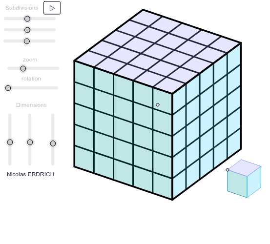
This example demonstrates how to construct volume models by transforming polygons and visualizing the changes. Core math concepts include volume calculation, matrix transformations, trigonometry, parallelograms, and similarity transformations. Construction highlights the use of GeoGebra commands like Sequence, Element, Polygon, Segment, and Translate. Suitable for high school and above students studying solid geometry, linear algebra, and transformation geometry.
GeoGebra Commands & Parameters
Sequence(Mat * Element[cube, k], k, 1, 8) → cube'Sequence(I + (Element[cube', k, 1, 1], Element[cube', k, 2, 1]), k, 1, 8) → listepointsElement(listepoints, 7) → FElement(listepoints, 6) → B_3Element(listepoints, 1) → EElement(listepoints, 2) → AElement(Element[AE, 3], 1) → droiteElement(listepoints, 4) → C_1Element(listepoints, 3) → DPolygon(A, E, C_1, D) → poly1, a_1, b, c_1, dElement(listepoints, 8) → GElement(listepoints, 5) → HPolygon(B_3, F, G, H) → poly2, e, f, g, hElement(listepoints, 3) → CPolygon(F, C, A, B_3) → poly3, f_1, i, a_2, b_1Element(AB, 3, 1) → avantPolygon(C_1, G, H, E) → poly4, c_2, g_1, h_1, e_1Element(AC, 3, 1) → dessusPolygon(F, C, C_1, G) → poly5, f_2, c_3, c_4, g_2Polygon(A, B_3, H, E) → poly6, a_3, b_2, h_2, e_2Segment(E, A) → cSegment(A, C) → jSegment(A, B_3) → kSegment(C, C_1) → lSegment(C_1, E) → mSegment(A, B_3) → pSegment(B_3, H) → qSegment(H, E) → rSegment(H, G) → sSegment(B_3, F) → tSegment(G, C_1) → d_1Segment(F, G) → i_1Segment(F, C) → j_1Polygon(A, B_3, F', D') → poly7, a_4, b_3, f', d'Polygon(E, A, D'', C') → poly8, e_3, a_5, d'', c'Polygon(B_3, F'', G', H) → poly9, b_4, f'', g', h_3Polygon(H, G'', C''', E) → poly10, h_4, g'', c''', e_4Polygon(A_2, B_2, G'', C''') → poly11, a_6, b_5, g''_1, c'''_1Sequence(E + (A - E) * k / m_1, k, 0, m_1) → l_2Sequence(A + (B_3 - A) * k / k_1, k, 0, k_1) → l_1Sequence(H + (E - H) * k / k_1, k, 0, k_1) → l_4Sequence(B_3 + (H - B_3) * k / m_1, k, 0, m_1) → l_5Sequence(Segment[Element[l_1, k], Element[l_4, k_1 - k + 2]], k, 0, k_1) → s_1Sequence(G + (C_1 - G) * k / k_1, k, 0, k_1) → l_6Sequence(H + (G - H) * k / n_1, k, 0, n_1) → l_7Sequence(E + (C_1 - E) * k / n_1, k, 0, n_1) → l_8Sequence(Segment[Element[l_4, k], Element[l_6, k]], k, 0, k_1) → s_4Sequence(D + (C_1 - D) * k / m_1, k, 0, m_1) → l_9Sequence(D + (A - D) * k / n_1, k, 0, n_1) → l_{10}Sequence(B_3 + (F - B_3) * k / n_1, k, 0, n_1) → l_{12}Sequence(D + (F - D) * k / k_1, k, 0, k_1) → l_{11}Sequence(Segment[Element[l_{11}, k], Element[l_6, k_1 - k + 2]], k, 0, k_1) → s_7Sequence(Segment[Element[l_{11}, k], Element[l_1, k]], k, 0, k_1) → s_8Sequence(G + (F - G) * k / m_1, k, 0, m_1) → l_{13}Sequence(Segment[Element[l_2, k], Element[l_5, m_1 - k + 2]], k, 0, m_1) → s_2Sequence(Segment[Element[l_9, k], Element[l_2, m_1 - k + 2]], k, 0, m_1) → s_6Sequence(Segment[Element[l_{13}, k], Element[l_9, m_1 - k + 2]], k, 0, m_1) → s_{12}Sequence(Segment[Element[l_{13}, k], Element[l_5, m_1 - k + 2]], k, 0, m_1) → s_{11}Sequence(Segment[Element[l_{12}, k], Element[l_{10}, n_1 - k + 2]], k, 0, n_1) → s_9Sequence(Segment[Element[l_{12}, k], Element[l_7, k]], k, 0, n_1) → s_{10}Sequence(Segment[Element[l_7, k], Element[l_8, k]], k, 0, n_1) → s_3Sequence(Segment[Element[l_8, k], Element[l_{10}, n_1 - k + 2]], k, 0, n_1) → s_5Translate(A, Vector[A, J]) → U_ATranslate(U_A, Vector[1 / n_1 * Vector[A, C]]) → U_CTranslate(U_A, Vector[1 / k_1 * Vector[A, B_3]]) → U_BTranslate(U_B, Vector[1 / n_1 * Vector[A, C]]) → U_FPolygon(J, U_C, U_F, U_B) → poly12, j_2, u_c, u_f, u_bTranslate(U_A, Vector[1 / m_1 * Vector[A, E]]) → U_ETranslate(U_E, Vector[1 / n_1 * Vector[E, C_1]]) → U_C1Polygon(U_C, J, U_E, U_C1) → poly13, u_1, j_3, u_e, u_c1Translate(U_C1, Vector[1 / k_1 * Vector[C_1, G]]) → U_GPolygon(U_C, U_C1, U_G, U_F) → poly14, u_2, u_3, u_g, u_4Translate(U_E, Vector[1 / k_1 * Vector[E, H]]) → U_HPolygon(U_C1, U_G, U_H, U_E) → poly15, u_5, u_6, u_h, u_7Polygon(U_H, U_G, U_F, U_B) → poly16, u_8, u_9, u_{10}, u_{11}Polygon(U_H, U_B, U_A, U_E) → poly17, u_{12}, u_{13}, u_a, u_{14}
AI Drawing Prompt Reference
Draw a skewed hexahedron composed of six parallelogram faces, whose vertices are obtained by translating a base cube through a matrix transformation. First construct the transformed vertices, then connect them to form six quadrilateral faces. Next, divide the edges proportionally and connect corresponding division points to create internal grid lines, illustrating volume subdivision. The figure includes parallelograms, edge segments, and families of parallel lines, showing a three-dimensional perspective of geometric transformation.
The prompt above was compiled from the original drawing commands and is for reference only.