
Tennis Ball Curve
Loading the math board and drawing, please wait…
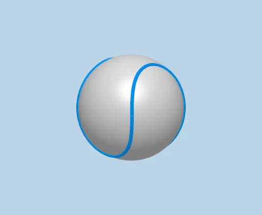
This example demonstrates the complex spatial curve generated when a tennis ball rotates. Key math concepts include spatial geometry, parametric equations, function graphing, and 3D visualization. Construction highlights involve commands like CurveCartesian, Sphere, and Point in GeoGebra. Suitable for high school and above students learning spatial geometry, parametric equations, and 3D graphing.
GeoGebra Commands & Parameters
CurveCartesian((r * cos(t)^(3)), (r * sin(t)^(3)), ((r * sqrt(3) / 2) * sin((2 * t))), t, 0, (2 * π)) → dSphere((0, 0, 0), r) → gPoint(d) → A
AI Drawing Prompt Reference
Draw a complex spatial curve generated by a rotating tennis ball. First, draw a sphere with radius r centered at the origin. Then, use parametric equations to draw the curve: x = r * cos(t)^3, y = r * sin(t)^3, z = (r * sqrt(3) / 2) * sin(2 * t), with t ranging from 0 to 2π.
The prompt above was compiled from the original drawing commands and is for reference only.