Square Root and Sum: Exploring Distances and Variance in Dynamic Geometry

Loading the math board and drawing, please wait…

2017-05-29 00:25

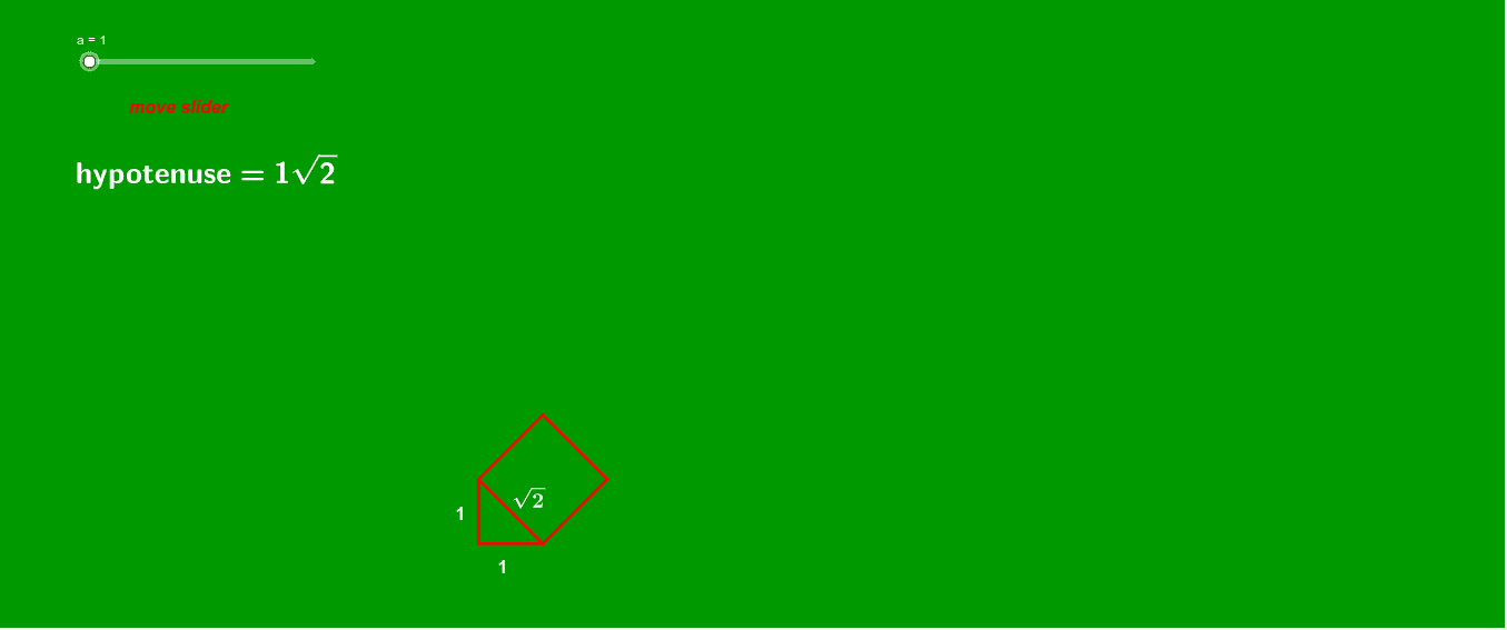
This GeoGebra example demonstrates the relationship between square root operations and sums of distances within a dynamic geometric construction, integrating concepts such as variance, reflection, and tangent lines. The core visualization involves multiple polygons, circles, segments, and auxiliary elements constructed via points, lines, intersections, midpoints, and perpendiculars. Key measurements (e.g., distances EG, BC, EB) are computed and displayed as text objects, allowing users to see how algebraic expressions like square roots and sums correspond to geometric quantities. The construction uses commands including Point, Line, Segment, Polygon, Circle, Intersect, Distance, Midpoint, and OrthogonalLine, building a rich network of objects labeled A through K and polygons poly1, poly2, poly3. This resource is suitable for high school or early college students studying distance formulas, square root functions, variance, and introductory differential calculus, offering a hands-on way to explore the interplay between algebra and geometry.

GeoGebra Commands & Parameters

Point(yAxis) → A
Line(A, xAxis) → a_1
Point(Circle[B, a]) → C
Segment(B, C) → c_2
Polygon(B, C, 4) → poly1, d, e, f, g, D, E
Line(E, C) → h
Circle(E, b) → k
Intersect(k, h) → F, G
Polygon(E, G, 4) → poly2, i, j, l, m, H, I
Distance(E, G) → distanceEG
Distance(B, C) → distanceBC
Distance(E, B) → distanceEB
Point(Circle[J, a]) → K
Segment(J, K) → p
Polygon(J, K, 4) → poly3, q, r, s, t, L, M
Polygon(M, K, 4) → poly4, b_1, c_1, d_1, e_1, N, O
Distance(J, K) → distanceJK
Distance(J, M) → distanceJM
Distance(M, K) → distanceMK
Distance(K, N) → distanceKN
Midpoint(M, K) → P
Midpoint(K, N) → Q
Midpoint(J, K) → R
Midpoint(J, M) → S
Segment(S, P) → f_1
Segment(P, R) → g_1
Midpoint(M, O) → T
Midpoint(O, N) → U
Segment(T, Q) → h_1
Segment(P, U) → i_1
Intersect(p, q) → V
Intersect(p, q) → W
Intersect(p, q) → Z
Circle(J, 1) → c
Circle(J, 2) → k_1
Intersect(c, q) → A_1,
Intersect(t, poly3) → B_1, C_1
Intersect(k_1, q) → D_1,
Intersect(t, poly3) → E_1, F_1
Intersect(k_1, t) → G_1,
Intersect(c, t) → H_1,
OrthogonalLine(D_1, p) → j_1
OrthogonalLine(A_1, p) → l_1
OrthogonalLine(H_1, t) → m_1
OrthogonalLine(G_1, t) → n_1
Intersect(n_1, b_1) → I_1
Intersect(m_1, b_1) → J_1
OrthogonalLine(J_1, b_1) → p_1
OrthogonalLine(I_1, b_1) → q_1
Intersect(c_1, m_1) → K_1
Intersect(c_1, n_1) → L_1
OrthogonalLine(K_1, c_1) → r_1
OrthogonalLine(L_1, c_1) → s_1
Midpoint(R, K) → M_1
OrthogonalLine(M_1, p) → t_1
Midpoint(S, M) → N_1
OrthogonalLine(N_1, t) → a_2
Intersect(e_1, t_1) → O_1
OrthogonalLine(O_1, e_1) → b_2
Intersect(poly3, poly4) → P_1, Q_1, R_1, S_1, T_1, U_1, V_1, W_1
Intersect(b_1, a_2) → Z_1
OrthogonalLine(Z_1, b_1) → d_2
Intersect(d_1, d_2) → A_2
Intersect(d_1, p_1) → B_2
Intersect(b_2, c_1) → C_2
Segment(N_1, Z_1) → e_2
Segment(Z_1, A_1) → f_2
Segment(H_1, J_1) → g_2
Segment(J_1, M_1) → h_2
Segment(J_1, B_2) → i_2
Segment(Z_1, A_2) → j_2
Segment(O_1, C_2) → k_2
Intersect(r_1, e_1) → D_2
Segment(D_2, K_1) → l_2
Segment(M, O) → m_2
Segment(O, N) → n_2
Segment(N, K) → p_2
Segment(K, M) → q_2
Segment(M, J) → r_2
Segment(J, K) → s_2
Segment(D_1, J_1) → t_2
Segment(A_1, I_1) → a_3
Segment(G_1, I_1) → b_3
Segment(H_1, J_1) → c_3
Segment(M, K) → d_3
Segment(M, J) → e_3
OrthogonalLine(I_1, d_3) → f_3
Segment(O, N) → h_3
Segment(M, O) → i_3
OrthogonalLine(L_1, p_2) → k_3
Intersect(k_3, i_3) → E_2
Intersect(f_3, h_3) → F_2
Segment(D_2, K_1) → g_3
Segment(E_2, L_1) → j_3
Segment(J_1, B_2) → l_3
Segment(I_1, F_2) → m_3
Segment(S, P) → n_3
Segment(P, R) → p_3
Segment(P, U) → q_3
Segment(T, Q) → r_3
Circle(J, 3) → s_3
Circle(J, 4) → t_3
Intersect(s_3, p) → G_2,
Intersect(t_3, p) → H_2,
Intersect(s_3, r_2) → I_2,
Intersect(t_3, r_2) → J_2,
OrthogonalLine(J_2, r_2) → a_4
OrthogonalLine(I_2, r_2) → b_4
OrthogonalLine(I_2, r_2) → c_4
OrthogonalLine(G_1, r_2) → d_4
OrthogonalLine(H_1, r_2) → e_4
Intersect(a_4, q_2) → K_2
Intersect(a_4, p_2) → L_2
Intersect(b_4, c_4) → M_2
Intersect(q_2, b_4) → N_2
Intersect(p_2, b_4) → O_2
OrthogonalLine(N_2, n_2) → f_4
OrthogonalLine(K_2, q_2) → g_4
OrthogonalLine(L_2, p_2) → h_4
OrthogonalLine(O_2, p_2) → i_4
Intersect(m_2, h_4) → P_2
Intersect(i_4, m_2) → Q_2
Intersect(n_2, f_4) → R_2
Intersect(g_4, n_2) → S_2
Segment(D_2, K_1) → j_4
Segment(E_2, L_1) → k_4
Segment(Q_2, O_2) → l_4
Segment(P_2, L_2) → m_4
Segment(F_2, I_1) → n_4
Segment(B_2, J_1) → p_4
Segment(J_1, H_2) → q_4
Segment(I_1, G_2) → r_4
Segment(N_2, D_1) → s_4
Segment(K_2, A_1) → t_4
Segment(H_1, J_1) → a_5
Segment(G_1, I_1) → b_5
Segment(I_2, N_2) → c_5
Segment(J_2, K_2) → d_5
Segment(K_2, S_2) → e_5
Segment(R_2, N_2) → f_5
Point(q_2) → T_2
Point(q_2) → U_2
Point(q_2) → V_2
Point(q_2) → W_2
Point(q_2) → Z_2
Point(r_2) → A_3
Point(p) → B_3
Point(q_2) → C_3
Point(q_2) → D_3
Point(q_2) → E_3
Point(q_2) → F_3
Point(r_2) → G_3
Point(p) → H_3
Point(q_2) → I_3
Point(q_2) → J_3
Point(q_2) → K_3
Point(r_2) → L_3
Point(p) → M_3
Point(q_2) → N_3
Point(q_2) → O_3
Point(r_2) → P_3
Point(p) → Q_3
Point(q_2) → R_3
Point(r_2) → S_3
Point(p) → T_3