
Spring Mass System Demonstration: Differential Equation and Geometric Constructi
Loading the math board and drawing, please wait…
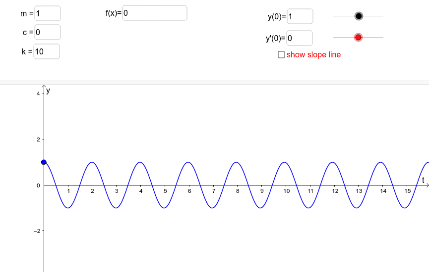
This example demonstrates the dynamic behavior of a spring-mass system, showing the application of differential equations in geometric graphics. Key mathematical concepts include differential equations, geometric construction, and parametric equations. Construction involves using GeoGebra commands such as Line, ComplexRoot, SolveODE, etc. to build the system model. Suitable for high school students or undergraduate students learning differential equations and geometric construction.
GeoGebra Commands & Parameters
Line(A, A + (1, initialY')) → eComplexRoot(charPoly) → z, wIf(y(z) ≟ 0, "" + (x(z)), "" + z) → zTextSolveODE((2 * p), w2, f, initialX, initialY, initialY', endX, step) → DEIf(y(w) ≟ 0, "" + (x(w)), "" + w) → wTextIf(dampTest < 0, "(underdamped)", If[dampTest > 0, "(overdamped)", "(critically damped)"]) → text5Textfield(m) → inputBox1Textfield(k) → inputBox3Textfield(c) → inputBox2First(DE, Length[DE]) → list1Textfield(f) → inputBox4Textfield(initialY) → inputBox5Textfield(initialY') → inputBox6
AI Drawing Prompt Reference
Create a dynamic demonstration of a spring-mass system showing the application of differential equations in geometric graphics. Include a spring and a mass point, with sliders to adjust parameters like mass, spring constant, and damping coefficient. Solve the system's motion using differential equations and display the trajectory through geometric construction, highlighting underdamped, overdamped, and critically damped states.
The prompt above was compiled from the original drawing commands and is for reference only.