Spherical Coordinates: Interactive 3D Visualization

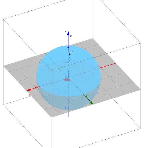
① This GeoGebra example dynamically illustrates a point P in 3D space using spherical coordinates, showing how radial distance ρ, polar angle φ, and azimuthal angle θ determine its position. ② Core mathematical concepts include the spherical coordinate system, conversion between Cartesian and spherical coordinates, and spatial geometry involving angles, distances, and projections. ③ Construction details: The Segment command creates coordinate axes and auxiliary segments, while Angle marks key angles; objects include variables ρ, φ, θ, point P and its projection P', auxiliary lines L, Lperp, Lpara, and equation eq1, all adjustable via sliders or input. ④ Suitable for upper high school or early university students learning multivariable calculus, 3D analytic geometry, or physics field theory, and for teachers demonstrating spatial coordinate systems in class.