
Sphere Animation
Loading the math board and drawing, please wait…
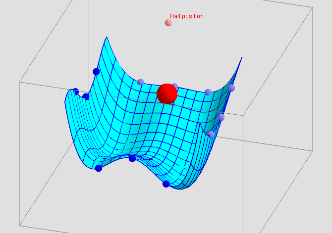
This example demonstrates a sphere animation. It involves concepts of spherical geometry and parametric equations. Using GeoGebra commands such as Surface, Sphere, and Sequence, a dynamic sphere model can be constructed. Suitable for high school and above students or teachers for teaching and learning solid geometry.
GeoGebra Commands & Parameters
Point(Line[(-1, -2, 0), (-1, -2, 1)]) → BPoint(Line[(0, -2, 0), (0, -2, 1)]) → CPoint(Line[(1, -2, 0), (1, -2, 1)]) → DPoint(Line[(-2, -1, 0), (-2, -1, 1)]) → FPoint(Line[(-2, 0, 0), (-2, 0, 1)]) → GPoint(Line[(-2, 1, 0), (-2, 1, 1)]) → HFitPoly({(x(A), z(A)), (x(B), z(B)), (x(C), z(C)), (x(D), z(D)), (x(E), z(E))}, 4) → fFitPoly({(y(A), z(A)), (y(F), z(F)), (y(G), z(G)), (y(H), z(H)), (y(I), z(I))}, 4) → gCurveCartesian(t, -2, f(t), t, -2, 2) → aCurveCartesian(-2, t, g(t), t, -2, 2) → bPoint(Line[(-1, 2, 0), (-1, 2, 1)]) → JPoint(Line[(0, 2, 0), (0, 2, 1)]) → KPoint(Line[(1, 2, 0), (1, 2, 1)]) → LFitPoly({(x(I), z(I)), (x(J), z(J)), (x(K), z(K)), (x(L), z(L)), (x(M), z(M))}, 4) → f2CurveCartesian(t, 2, f2(t), t, -2, 2) → dPoint(Line[(2, -1, 0), (2, -1, 1)]) → NPoint(Line[(2, 0, 0), (2, 0, 1)]) → OPoint(Line[(2, 1, 0), (2, 1, 1)]) → PFitPoly({(y(E), z(E)), (y(N), z(N)), (y(O), z(O)), (y(P), z(P)), (y(M), z(M))}, 4) → g2CurveCartesian(2, t, g2(t), t, -2, 2) → eSurface(u, v, ((1 - (v + 2) / 4) * f(u)) + ((v + 2) / 4 * f2(u)) + ((1 - (u + 2) / 4) * g(v)) + ((u + 2) / 4 * g2(v)), u, -2, 2, v, -2, 2) → cPlane(Q', Plx, Ply) → iOrthogonalLine(Q', i) → jIntersect(j, Sphere[Q', r]) → S, TSphere(T, r) → k_1Sequence(CurveCartesian[u, v, ((1 - (v + 2) / 4) * f(u)) + ((v + 2) / 4 * f2(u)) + ((1 - (u + 2) / 4) * g(v)) + ((u + 2) / 4 * g2(v)), u, -2, 2], v, -2, 2, 4 / n) → liste1Sequence(CurveCartesian[u, v, ((1 - (v + 2) / 4) * f(u)) + ((v + 2) / 4 * f2(u)) + ((1 - (u + 2) / 4) * g(v)) + ((u + 2) / 4 * g2(v)), v, -2, 2], u, -2, 2, 4 / n) → liste2
AI Drawing Prompt Reference
Create an animation of a sphere to demonstrate its dynamic changes. First, create several points on lines at different positions, then fit four polynomial curves based on these points. Next, generate two curves using these curves, and construct a surface from them. Finally, create multiple curves on the surface to form the dynamic effect of the sphere.
The prompt above was compiled from the original drawing commands and is for reference only.