
Solving Linear Equations via Transformations
Loading the math board and drawing, please wait…
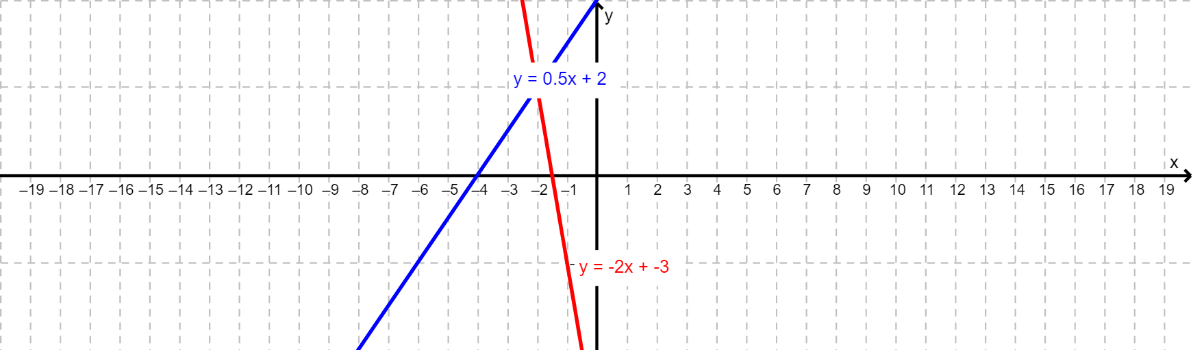
This example demonstrates how to solve systems of linear equations visually using geometric transformations. Key math concepts include linear equations, transformations, and intersection points. It utilizes GeoGebra commands and objects such as Textfield, Intersect, Step, m_2, b_1, m_1, b_2, inputBoxm_1, inputBoxb_1, inputBoxm_2, inputBoxb_2, Transform_5, NoSolution, equalsX, AnyReal, Transform_1, Space, Comma, reset, Yzoom, Xzoom, Transform_3, Transform_2, trans5, Transform_4, trans1, trans3, trans2, trans4, f1, f2, fa, c, F1x, F1y, F1x_1, F1y_1, F2x, F2x_1, F2y, F2y_1, Fax. Suitable for high school mathematics teaching and self-learning, helping students understand the geometric meaning and solution steps of linear equation systems.
GeoGebra Commands & Parameters
Textfield(m_1) → inputBoxm_1Textfield(b_1) → inputBoxb_1Textfield(m_2) → inputBoxm_2Textfield(b_2) → inputBoxb_2Intersect(f1, x = (0.7 * Xzoom), (14, 9)) → F1xIntersect(f1, y = (0.7 * Yzoom), (-1.2000000000000002, 1.4)) → F1yIntersect(f1, x = (-0.7 * Xzoom), (-14, -5)) → F1x_1Intersect(f1, y = (-0.7 * Yzoom), (-6.8, -1.4)) → F1y_1Intersect(f2, x = (0.7 * Xzoom), (14, -31)) → F2xIntersect(f2, x = (-0.7 * Xzoom), (-14, 25)) → F2x_1Intersect(f2, y = (0.7 * Yzoom), (-2.2, 1.4)) → F2yIntersect(f2, y = (-0.7 * Yzoom), (-0.8, -1.4)) → F2y_1Intersect(fa, x = (0.7 * Xzoom), (14, 9)) → FaxIntersect(fa, x = (-0.7 * Xzoom), (-14, -5)) → Fax_1Intersect(fa, y = (0.7 * Yzoom), (-1.2000000000000002, 1.4)) → FayIntersect(fa, y = (-0.7 * Yzoom), (-6.8, -1.4)) → Fay_1