
Solve System of Equations Practice y=mx+b V2
Loading the math board and drawing, please wait…
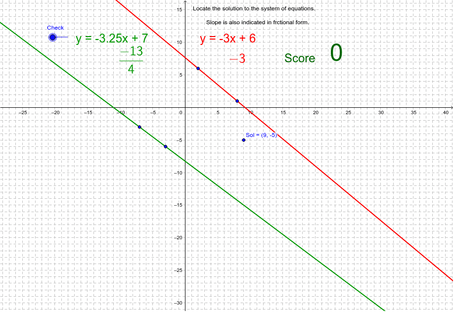
This example demonstrates how to solve systems of linear equations using GeoGebra, where the equations are in the form y=mx+b. Core mathematical concepts include linear functions, slope, y-intercept, and methods for solving systems of equations. Key GeoGebra commands and objects used are Random, If, Line, Text, FractionText, etc., to dynamically adjust parameters and visually show the geometric meaning of solutions. Suitable for high school students learning analytical geometry and function graphs.
GeoGebra Commands & Parameters
Random(1, 10) → aaRandom(-10, 10) → bRandom(0, 1) → sIf(s ≟ 0, -1, 1) → snRandom(-10, 10) → rRandom(-10, 10) → gLine(R, B) → RedLine(G, B) → GreenLine(A, C) → cLine(D, E) → dIf(Sol ≟ B, 1, 0) → addptText(Red) → text2Text(Green) → text3FractionText(slopered) → text4FractionText(slopegreen) → text5Text(score) → text8
AI Drawing Prompt Reference
Draw two lines, one red and one green, representing two linear equations y=mx+b with random slopes of 1 or -1 and random intercepts, label the slope and intercept of each line with text, mark the intersection point of the two lines with a special symbol, and display the slope values in fractional form.
The prompt above was compiled from the original drawing commands and is for reference only.