
Solution to a System of Linear Inequalities
Loading the math board and drawing, please wait…
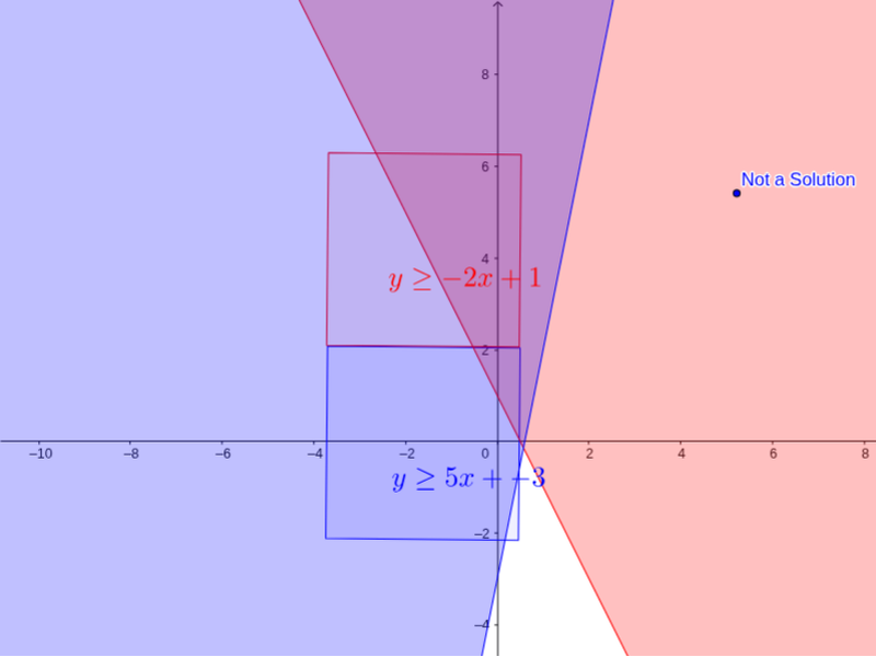
This example shows how to use GeoGebra to dynamically graph a system of linear inequalities and visualize its solution region. It covers graphing linear inequalities, slope‑intercept form, intersection of half‑planes, and the effect of varying parameters via sliders on the feasible region. The GeoGebra construction employs DynamicCoordinates to keep points updated in real time and uses a Polygon to shade the region satisfying all inequalities. Designed for high school algebra, college calculus‑ready courses, and any class covering linear programming or visual mathematics.
GeoGebra Commands & Parameters
DynamicCoordinates(A, x(A), y(A)) → BDynamicCoordinates(A, x(A), y(A)) → CDynamicCoordinates(A, x(A), y(A)) → DDynamicCoordinates(A, x(A), y(A)) → EDynamicCoordinates(A, x(A), y(A)) → FDynamicCoordinates(A, x(A), y(A)) → GDynamicCoordinates(A, x(A), y(A)) → HDynamicCoordinates(A, x(A), y(A)) → IDynamicCoordinates(A, x(A), y(A)) → JDynamicCoordinates(A, x(A), y(A)) → KDynamicCoordinates(A, x(A), y(A)) → LDynamicCoordinates(A, x(A), y(A)) → MDynamicCoordinates(A, x(A), y(A)) → NDynamicCoordinates(A, x(A), y(A)) → ODynamicCoordinates(A, x(A), y(A)) → PPolygon(Q, R, 4) → poly1, q, r, s, t, S, TPolygon(Q_1, R_1, 4) → poly1_1, q_1, r_1, s_1, t_1, S_1, T_1
AI Drawing Prompt Reference
Draw a graph showing the solution region of a system of linear inequalities. Start with two boundary lines, one in slope-intercept form and the other intersecting it. Shade the half-plane satisfying each inequality with a semi-transparent color, and highlight the overlapping area as the feasible region using a filled polygon. Include coordinate axes, grid lines, and dynamic sliders that adjust the slope or intercept of the lines, causing the feasible region to change shape and all intersection points to update in real time.
The prompt above was compiled from the original drawing commands and is for reference only.