
Solids of Revolution: Rotating a Region Between Two Functions
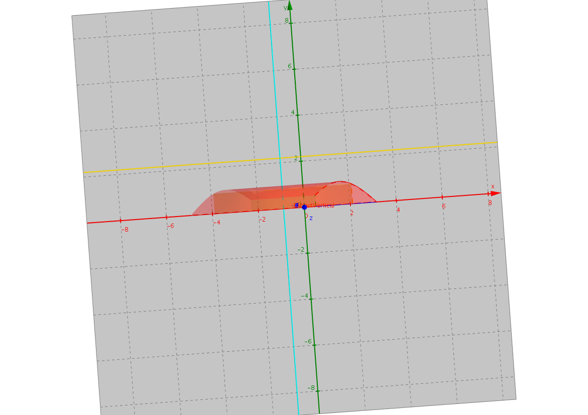
Loading the math board and drawing, please wait…
① This example demonstrates how to rotate a planar region bounded by two functions around a vertical or horizontal axis to create a 3D solid, and visualizes its volume and cross-sections. ② Core mathematical concepts include volume of solids of revolution via definite integrals (disk/washer or shell methods), function graphs, the relationship between 2D regions and 3D solids, and the effect of the axis of rotation on the resulting volume. ③ Construction details: The GeoGebra commands CurveCartesian define the two functions f and g, while Surface commands generate the rotated surfaces (e.g., fAboutVertical, gAboutVertical, fAboutHorizontal, gAboutHorizontal) around the vertical axis (vaxis) and horizontal axis (haxis). Rectangles (rectangle) and boundary edges (aEdge, bEdge) help visualize the original region, and sliders (Bound1, Bound2) control the integration limits for dynamic exploration. ④ This is suitable for high school advanced or university calculus courses, for teachers demonstrating the concept or students exploring how different functions and axes affect the volume.
GeoGebra Commands & Parameters
CurveCartesian(t, f(t), t, a, b) → f_pCurveCartesian(t, g(t), t, a, b) → g_pCurveCartesian(vaxis, t, t, -10, 10) → verticalSurface(vaxis + ((vaxis - t) * cos(u)), g(t), ((vaxis - t) * sin(u)), t, a, b, u, 0, 6.28319) → gAboutVerticalCurveCartesian(vrect, (t * f(vrect)) + ((1 - t) * g(vrect)), t, 0, 1) → rectangleSurface(vaxis + ((vrect - vaxis) * cos(u)), (t * f(vrect)) + ((1 - t) * g(vrect)), ((vrect - vaxis) * sin(u)), t, 0, 1, u, 0, 6.283185307179586) → RectangleAboutVerticalSurface(vaxis + ((vaxis - a) * cos(u)), (t * f(a)) + ((1 - t) * g(a)), ((vaxis - a) * sin(u)), t, 0, 1, u, 0, 6.283185307179586) → aEdgeAboutVerticalSurface(vaxis + ((vaxis - b) * cos(u)), (t * f(b)) + ((1 - t) * g(b)), ((vaxis - b) * sin(u)), t, 0, 1, u, 0, 6.28319) → bEdgeAboutVerticalSurface(t, haxis + ((f(t) - haxis) * cos(u)), ((f(t) - haxis) * sin(u)), t, a, b, u, 0, 6.283185307179586) → fAboutHorizontalSurface(t, haxis + ((g(t) - haxis) * cos(u)), ((g(t) - haxis) * sin(u)), t, a, b, u, 0, 6.283185307179586) → gAboutHorizontalSurface(b, haxis + ((t - haxis) * cos(u)), ((t - haxis) * sin(u)), t, Min[abs(f(b)), abs(g(b))], Max[abs(f(b)), abs(g(b))], u, 0, 6.28319) → bEdgeAboutHorizontalSurface(a, haxis + ((t - haxis) * cos(u)), ((t - haxis) * sin(u)), t, Min[abs(f(a)), abs(g(a))], Max[abs(f(a)), abs(g(a))], u, 0, 6.28319) → aEdgeAboutHorizontalCurveCartesian(t, haxis, t, -10, 10) → horizontalSurface(vrect, haxis + ((haxis - t) * cos(u)), ((haxis - t) * sin(u)), t, Min[abs(f(vrect)), abs(g(vrect))], Max[abs(f(vrect)), abs(g(vrect))], u, 0, 6.283185307179586) → RectangleAboutHorizontalCurveCartesian(a, (t * f(a)) + ((1 - t) * g(a)), t, 0, 1) → Bound1CurveCartesian(b, (t * f(b)) + ((1 - t) * g(b)), t, 0, 1) → Bound2Surface(vaxis + ((vaxis - t) * cos(u)), f(t), ((vaxis - t) * sin(u)), t, a, b, u, 0, 6.283185307179586) → fAboutVertical
AI Drawing Prompt Reference
Draw a 3D solid formed by rotating a planar region bounded by two functions f and g around a vertical or horizontal axis. First, plot the graphs of the two functions, then generate the surfaces of the rotated solid using the disk/washer and shell methods around the vertical and horizontal axes. Finally, use rectangles and boundary lines to visualize the original region, and control the rotation range with sliders to explore how different functions and axes affect the volume.
The prompt above was compiled from the original drawing commands and is for reference only.