
Slope Fields and Solution Curves
Loading the math board and drawing, please wait…
In collections
Differential Equations
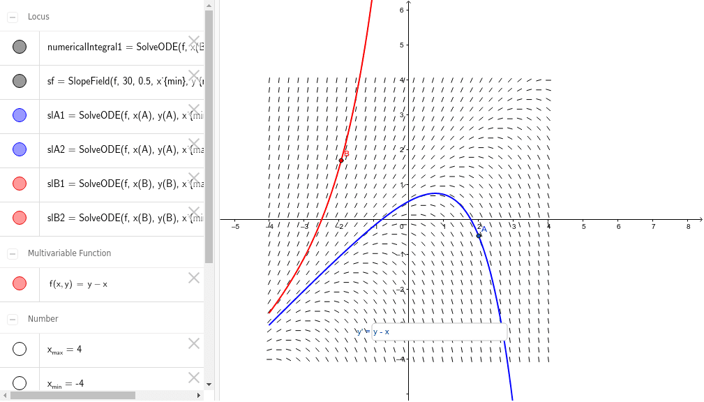
This example demonstrates the automatic creation of a slope field and the plotting of two solution curves. Key mathematical concepts include the solution of differential equations. GeoGebra commands used include SlopeField and SolveODE. Suitable for high school and above students learning the concept of slope fields in calculus.
GeoGebra Commands & Parameters
Textfield(f) → y'SlopeField(f, 30, 0.5, x_{min}, y_{min}, x_{max}, y_{max}) → sfSolveODE(f, x(B), y(B), x_{max}, 0.01) → numericalIntegral1SolveODE(f, x(B), y(B), x_{max}, 0.01) → slB1SolveODE(f, x(B), y(B), x_{min}, 0.01) → slB2SolveODE(f, x(A), y(A), x_{min}, 0.01) → slA1SolveODE(f, x(A), y(A), x_{max}, 0.01) → slA2
AI Drawing Prompt Reference
Create a slope field based on the function y', ranging from x_min to x_max and y_min to y_max. Use numerical integration to plot two solution curves, starting at points A and B, and ending at x_max and x_min.
The prompt above was compiled from the original drawing commands and is for reference only.