
Slope Field Generator by DNghiem
Loading the math board and drawing, please wait…
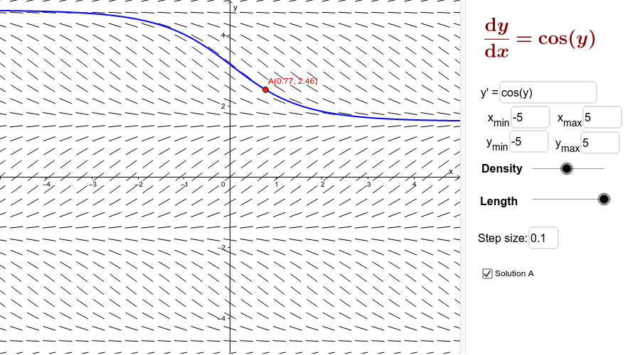
This example demonstrates how to generate slope fields for differential equations and plot approximate solution curves given initial values. Key math concepts include differential equations, derivatives, and integrals. Construction highlights: utilizes GeoGebra commands and objects like Textfield, SlopeField, SolveODE, f, inputBox, n, x_{min}, etc., to interactively show the dynamic behavior of slope fields and solution curves under different initial conditions. Suitable for high school and above students to learn the geometric interpretation of differential equations and methods for plotting solution curves.
GeoGebra Commands & Parameters
Textfield(f) → inputBox1Textfield(x_{min}) → inputBox2Textfield(x_{max}) → inputBox3Textfield(y_{min}) → inputBox4Textfield(y_{max}) → inputBox5SlopeField(f, n, L, x_{min}, y_{min}, x_{max}, y_{max}) → slopefield1Textfield(delta) → inputBox6SolveODE(f, x(A), y(A), x_{max}, delta) → numericalIntegral1SolveODE(f, x(A), y(A), (-x_{max}), delta) → numericalIntegral2SolveODE(f, x(B), y(B), x_{max}, delta) → numericalIntegral3SolveODE(f, x(B), y(B), x_{min}, delta) → numericalIntegral4SolveODE(f, x(C), y(C), x_{max}, delta) → numericalIntegral5SolveODE(f, x(C), y(C), x_{min}, delta) → numericalIntegral6SolveODE(f, x(D), y(D), x_{max}, delta) → numericalIntegral7SolveODE(f, x(D), y(D), x_{min}, delta) → numericalIntegral8
AI Drawing Prompt Reference
Draw a slope field for a differential equation and display several approximate solution curves. First, input the function expression and coordinate range to generate the slope field. Then, plot solution curves starting from four initial positions (lower left, upper left, upper right, lower right) to show the dynamic behavior of the function.
The prompt above was compiled from the original drawing commands and is for reference only.