Slope Field Demonstration

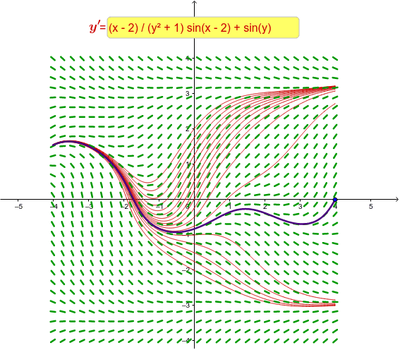
This example demonstrates the slope field of a differential equation, visually showing the direction of solution curves. It involves core mathematical concepts such as differential equations, slope fields, solution curves, and derivatives. Key GeoGebra commands and objects used include Textfield, SlopeField, SolveODE, Sequence, and elements like text1, f, inputBox1, A, x_{min}, etc. It is suitable for high school and university students learning the geometric interpretation of differential equations, or for introductory calculus teaching.