
Sketch a Cumulative Frequency Curve
Loading the math board and drawing, please wait…
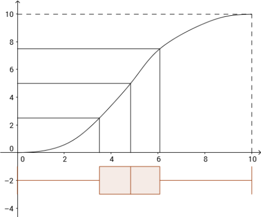
This GeoGebra example demonstrates how to construct a cumulative frequency curve, also known as an ogive, to visualize the cumulative count of data points as values increase. It integrates core statistical concepts such as frequency distribution, cumulative frequency, histograms, and box plots. The construction uses GeoGebra commands including Point to place data points, Spline to create a smooth curve, Intersect for finding intersections, Segment for auxiliary lines, BoxPlot and Histogram for statistical visualizations, Sum to compute cumulative totals, ParametricDerivative for analyzing curve derivatives, Sequence for generating ordered data, and Length for measuring segment lengths. This resource is ideal for middle and high school statistics lessons, as well as introductory college statistics courses, helping students understand how to build and interpret cumulative frequency curves from raw data.
GeoGebra Commands & Parameters
Point(x = Row[A1]) → B1Point(x = Row[A2]) → B2Point(x = Row[A3]) → B3Point(x = Row[A4]) → B4Point(x = Row[A5]) → B5Point(x = Row[A6]) → B6Point(x = Row[A7]) → B7Point(x = Row[A8]) → B8Point(x = Row[A9]) → B9Point(x = Row[A10]) → B10Spline(Append[B0, B1:B10], 3) → aIntersect(f, a) → A, A_1, A_2Intersect(h, a) → B, B_1, B_2Intersect(g, a) → C, C_1, C_2Segment((0, y(A)), A) → iSegment((0, y(B)), B) → jSegment((0, y(C)), C) → kSegment((x(A), 0), A) → lSegment((x(B), 0), B) → mSegment((x(C), 0), C) → pBoxPlot(-2, 1, 0, x(C), x(A), x(B), x(B10)) → cSegment((x(B10), 0), B10) → qSegment((0, y(B10)), B10) → rSum(D1:D10) → errorSegment(D, E) → tParametricDerivative(a) → sSequence(y(Intersect[x = (10 * i / n) + 5 / n, s]), i, 0, n - 1) → list7Length(list7) → dHistogram(list6, list7) → e
AI Drawing Prompt Reference
Draw a cumulative frequency curve (ogive) by plotting data points and connecting them with a smooth spline. At the intersections of this curve with three auxiliary lines (horizontal, vertical, and diagonal), draw perpendicular and horizontal segments to the axes. Below the curve, place a box plot showing the data spread. Additionally, construct a parametric derivative curve of the main curve, and at its intersections with equally spaced vertical lines, generate a sequence of points; use these points to create a histogram that reflects the rate of change in cumulative frequency. The final graph should include coordinate axes, data points, the smooth curve, intersection segments, a box plot, and a histogram, clearly illustrating the statistical distribution.
The prompt above was compiled from the original drawing commands and is for reference only.