
SIR Model Simulation for Simplified COVID-19 Dynamics
Loading the math board and drawing, please wait…
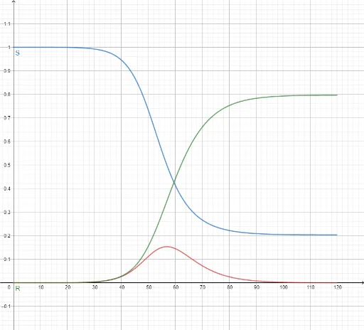
① This GeoGebra example demonstrates a simplified SIR (Susceptible-Infectious-Recovered) model for COVID-19 spread, showing how the three population compartments evolve over time through numerical solution of differential equations. ② Core mathematical concepts include systems of ordinary differential equations, population dynamics, exponential growth and saturation, and parameter sensitivity; the model tracks S, I, R with transmission rate (transm) and recovery rate (recov). ③ Construction highlights: the NSolveODE command numerically integrates the ODE system; initial values N, Istart, Sstart, Rstart and parameters transm, recov, maxT are defined; derivatives S', I', R' are computed, and the functions S, I, R are plotted against time. ④ Suitable for high school to undergraduate courses in mathematical modeling, biomathematics, or epidemiology, helping learners grasp the mathematical basis of disease spread and how adjusting parameters affects epidemic curves.
GeoGebra Commands & Parameters
NSolveODE({S', I', R'}, 0, {Sstart, Istart, Rstart}, maxT) → S, I, R
AI Drawing Prompt Reference
Create a graph showing the SIR model for simplified COVID-19 spread, with curves of S, I, R populations evolving over time obtained via numerical solution of differential equations, initial values and parameters like transmission and recovery rates, along with a time range, are set, and demonstrate the effect of adjusting parameters on the epidemic curves.
The prompt above was compiled from the original drawing commands and is for reference only.