Sine Graph with Unit Circle Dynamic Demonstration

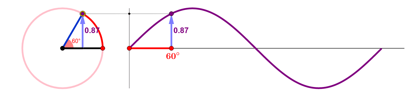
①This example visually demonstrates how the sine function graph is generated by linking a moving point on the unit circle to its corresponding point on the sine curve, connecting angle changes to function values. ②Core mathematical concepts include trigonometric functions (sine and cosine), the unit circle, angle-radian correspondence, and the locus of function graphs. ③Construction highlights: using GeoGebra commands such as Point, Circle, Angle, Segment, Arc, Locus, Vector, CurveCartesian, and Text, it builds a unit circle, angle α, moving point P, and generates the sine curve f via Locus, with text labels for key points and values, enabling dynamic interaction. ④Suitable for high school trigonometry lessons, pre-calculus review, and math enthusiasts exploring the geometric intuition behind function graphs, as well as for teachers creating interactive materials.