
Sine Function Transformation
Loading the math board and drawing, please wait…
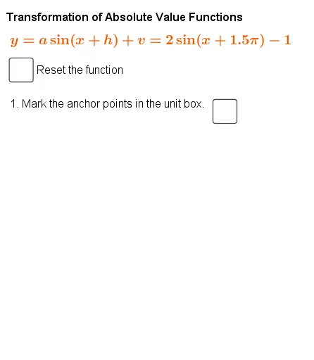
This example demonstrates the transformation process of the sine function, allowing users to dynamically adjust parameters and observe changes in the function's graph. Key math concepts include function transformations, amplitude, period, and phase shifts. Constructed using GeoGebra commands like Point, RandomElement, Random, Element, If, and Polygon. Suitable for high school mathematics students to learn and understand the properties of function graph transformations, as well as for calculus instruction on function analysis.
GeoGebra Commands & Parameters
Point(k) → C1RandomElement(KeepIf[x ≠ 0, Sequence[i, i, ymin + 2, ymax - 2 + If[reset, 0, 0]]]) → aRandom(1, 7 + If[reset, 0, 0]) → hElement(hh, h) → hhhRandom(ymin + abs(a), ymax - abs(a) + If[reset, 0, 0]) → vRandom(2, 9 + If[reset, 0, 0]) → nIf(Mod[n, 2] ≟ 0, 1, -1) → eoPolygon(A, B, C, D) → q1, a_1, b_1, c, dPolygon((x(C0), y(C1m)), (x(C0), y(C3)), (x(C4), y(C3)), (x(C4), y(C1m))) → q2, g, i, j, k_1
AI Drawing Prompt Reference
Draw a sine function transformation diagram showing how the graph changes as parameters are adjusted dynamically, including amplitude, period, and phase shift. Include a point, several randomly generated auxiliary points and line segments, and two polygons forming the upper and lower envelopes and partial outlines of the function graph to illustrate the transformation effects.
The prompt above was compiled from the original drawing commands and is for reference only.