
Self-Assessment: Quadratic Function Graphs
Loading the math board and drawing, please wait…
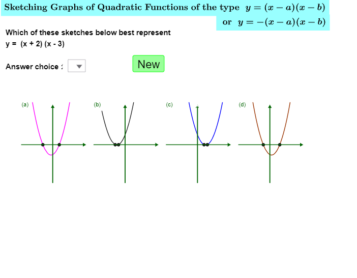
This example demonstrates the plotting and transformation of quadratic function graphs, focusing on vertex, axis of symmetry, and direction of opening variations. Key math concepts include quadratic functions, vertex form (x-a)(x-b), symmetry, and coefficient effects. GeoGebra commands like Random, If, Shuffle, Coefficients, Element, Sequence, Polygon, Defined, Min, Max are used to dynamically generate and adjust function parameters. Suitable for high school mathematics teaching, enabling students to explore the properties of quadratic function graphs and parameter relationships independently.
GeoGebra Commands & Parameters
Random(1, 4) → dRandom(2, 4) → e'If(d ≟ e' ∧ (count > 7 ∨ count < 5), 1, e') → eShuffle({2, 6, 7, 8}) → listshowFf2b, {8, 6, 2, 7}Shuffle({1, 4, 5, 8}) → listshowFf2a, {5, 4, 1, 8}Shuffle({1, 2, 3, 4}) → listshowFf1, {3, 4, 1, 2}If(count < 4, Element[listFf, Element[listshowFf1, 2]], If[count < 8, Element[listFf, Element[listshowFf2a, 2]], Element[listFf, Element[listshowFf2b, 2]]]) → f_{2s}Random(1, 4) → n_fCoefficients(f_{2s}) → listf_{2s}If(count < 4, Element[listFf, Element[listshowFf1, 1]], If[count < 8, Element[listFf, Element[listshowFf2a, 1]], Element[listFf, Element[listshowFf2b, 1]]]) → f_{1s}If(count < 4, Element[listFf, Element[listshowFf1, 4]], If[count < 8, Element[listFf, Element[listshowFf2a, 4]], Element[listFf, Element[listshowFf2b, 4]]]) → f_{4s}Coefficients(f_{1s}) → listf_{1s}Coefficients(f_{4s}) → listf_{4s}If(count < 4, Element[listFf, Element[listshowFf1, 3]], If[count < 8, Element[listFf, Element[listshowFf2a, 3]], Element[listFf, Element[listshowFf2b, 3]]]) → f_{3s}Coefficients(f_{3s}) → listf_{3s}Element(listCoeffs, n_f, 2) → b_fElement(listCoeffs, n_f, 1) → a_fSequence(Sequence[(x(A) + (s_p * i), y(A) + (s_p * j)), i, 0, 3], j, 0, 0) → list3CtrofGraphs, {{(5, 0), (13.8, 0), (22.6, 0), (31.400000000000002, 0)}}Polygon(E, D, F, G) → poly2, e_1, d_1, f_5, gPolygon(G, F, H, I) → poly3, g_1, f_6, h, iPolygon(J, K, L, M) → poly4, j, k, l, mPolygon(J, K, C, B) → poly5, j_1, k_1, c, b_1Sequence(Sequence[Segment[(x(A) + (s_p * i) - l_x / 2, y(A) + (s_p * j)), (x(A) + (s_p * i) + l_x / 2, y(A) + (s_p * j))], i, 0, 3], j, 0, 0) → list1Xaxes, {{7.6000000000000005, 7.600000000000001, 7.600000000000001, 7.600000000000001}}Sequence(Sequence[Segment[(x(A) + (s_p * i), y(A) + (s_p * j) - l_y / 2), (x(A) + (s_p * i), y(A) + (s_p * j) + l_y / 2)], i, 0, 3], j, 0, 0) → list2Yaxes, {{9.2, 9.2, 9.2, 9.2}}Sequence(Sequence[(x(A) + l_x / 2 + (s_p * i), y(A) + (s_p * j)), i, 0, 3], j, 0, 0) → listXarrow, {{(8.8, 0), (17.6, 0), (26.400000000000002, 0), (35.2, 0)}}Sequence(Sequence[(x(A) + (s_p * i), y(A) + l_y / 2 + (s_p * j)), i, 0, 3], j, 0, 0) → listYarrow, {{(5, 4.6), (13.8, 4.6), (22.6, 4.6), (31.400000000000002, 4.6)}}Sequence(Sequence[Text[Element[listChoicestext, i + 1], (x(A) - l_x / 2 + (s_p * (i - 1)), y(A) + l_y / 2)], i, 1, 4], j, 0, 0) → listChoicestextDisplay, {{"(a)", "(b)", "(c)", "(d)"}}Element(listCoeffs, n_f, 3) → c_fDefined(root1) → realrootsIf(count < 4, Element[listFf, Element[listshowFf1, 4]], If[count < 8, Element[listFf, Element[listshowFf2a, 4]], Element[listFf, Element[listshowFf2b, 4]]]) → f_{tests}Polygon(B, C, D, E) → poly1, b, c_1, d_2, e_2If(count < 5, Element[listshowFf1, n_f], If[count < 9, Element[listshowFf2a, n_f], Element[listshowFf2b, n_f]]) → n_sSequence(If[count < 4, Element[listshowFf1, i], If[count < 8, Element[listshowFf2a, i], Element[listshowFf2b, i]]], i, 1, 4) → listnsSequence({Cell[9, Element[listns, i]], Cell[10, Element[listns, i]]}, i, 1, 4) → listfsrootsSequence(Sequence[(((Element[listfsroots, i, j] * 2) * f_s) + x(A) + (s_p * (i - 1)), y(A)), j, 1, 2], i, 1, 4) → listfsxinttrans, {{(3.8, 0), (5.8, 0)}, {(12.600000000000001, 0), (13, 0)}, {(23.400000000000002, 0), (23.8, 0)}, {(30.6, 0), (32.6, 0)}}Min(d, e) → I1Min((-d), e) → I2Min(d, (-e)) → I3Min((-d), (-e)) → I4Min(d, e) → I5Min((-d), e) → I6Min(d, (-e)) → I7Min((-d), (-e)) → I8Max(d, e) → J1Max((-d), e) → J2Max((-d), e) → J6Max(d, (-e)) → J7Max(d, (-e)) → J3Max((-d), (-e)) → J4Max(d, e) → J5Max((-d), (-e)) → J8Element(listTurningPoints, n_f) → T_{do}Sequence(Sequence[(Element[listfsroots, i, j], y(A)), j, 1, 2], i, 1, 4) → listfsxintbeforetrans, {{(-3, 0), (2, 0)}, {(-3, 0), (-2, 0)}, {(2, 0), (3, 0)}, {(-2, 0), (3, 0)}}Element(listfsxintbeforetrans, n_f, 1) → R_{1o}Element(listfsxintbeforetrans, n_f, 2) → R_{2o}Element(listfsxinttrans, n_f, 1) → R_{1}Element(listfsxinttrans, n_f, 2) → R_{2}Element(listfYint, n_f) → Y_{into}