
Sections of a Cone (G.GGMD.4)
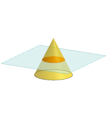
Loading the math board and drawing, please wait…
This interactive GeoGebra example demonstrates the different conic sections obtained by cutting a cone with a plane, including circles, ellipses, parabolas, and hyperbolas. The core mathematical concepts involve solid geometry, the definition of conic sections, and how the relative position of the cutting plane to the cone's axis and surface determines the resulting curve. Construction highlights: the cone is created using the Cone command, a cutting plane is defined with the Plane command, and the intersection curve is computed via IntersectPath. Additional commands such as Rotate, Translate, OrthogonalLine, PointIn, and Polygon are used to manipulate the plane and construct auxiliary points and polygons, while multiple text objects dynamically label the type of section. This resource is suitable for high school or early college students to visually explore the geometric origins of conic sections, and for teachers to use in classroom demonstrations or guided inquiry.
GeoGebra Commands & Parameters
Polygon(B + (-2, -2), B + (2, -2), B + (2, 2), B + (-2, 2)) → poly3, e, f, g, iPointIn(poly3) → CTranslate((0, 0, 0), Vector[B, C]) → APolygon(A + (-4, -4), A + (4, -4), A + (4, 4), A + (-4, 4)) → poly1, a, b, c, dRotate(Rotate[Translate[poly1, Vector[A, A + (0, 0, h)]], (90° * s), A + (0, 0, h), yAxis], (90° * t), A, zAxis) → poly2Rotate(D, 120°, (0, 0, 0)) → ECone((0, 0, 0), (0, 0, 4), 2) → m, e_1, oPolygon(D, E, 3, xOyPlane) → poly4, j, k, l, FPointIn(poly2) → GPointIn(poly2) → HPointIn(poly2) → IPlane(G, I, H) → nIntersectPath(n, m) → poly6OrthogonalLine(A, n) → d_1Ends(m) → g_1, g_1_1