
Scatterplot and Residual Plot
Loading the math board and drawing, please wait…
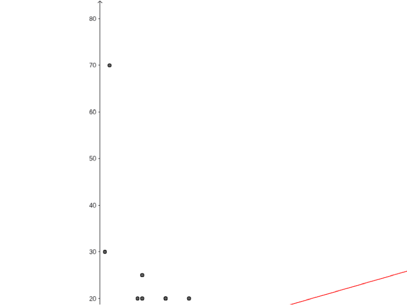
This example demonstrates how to compare the relationship between AP classes taken and study time using a scatter plot, and analyze data fitting by creating a residual plot. Key math concepts include statistical graphs, linear regression, and residual analysis. The construction involves commands like FitLineY and ResidualPlot with data points A1-B20. Suitable for high school and above mathematics and statistics courses for data analysis and model evaluation.
GeoGebra Commands & Parameters
FitLineY(list1) → bFitLineY(list2) → cResidualPlot({(4, 17), (19, 20), (1, 10), (2, 11), (3, 8), (6, 8), (0, 2), (1, 30), (0, 8), (0, 0.5), (9, 20), (9, 25), (5, 15), (0, 10), (8, 20), (9, 5), (8, 5), (6, 0), (3, 2), (9, 7), (2, 7), (6, 10), (9, 13), (4, 10), (1, 7), (3, 4), (1, 10), (1, 4), (2, 4), (11, 12), (1, 5), (2, 6), (5, 10), (5, 4), (0, 5), (12, 3), (2, 10), (6, 15), (8, 6), (1, 3), (8, 5), (2, 5), (0, 2), (8, 7), (0, 3), (8, 3), (14, 20), (12, 15), (12, 8), (1, 0), (14, 20), (3, 4), (0, 0), (6, 1), (4, 7), (10, 10), (6, 0), (0, 2), (15, 15), (2, 6), (2, 5), (3, 15), (8, 8), (8, 8), (7, 5), (7, 10), (14, 4), (16, 10), (20, 12), (5, 5), (2, 4), (8, 8), (11, 12), (2, 70), (1, 0), (10, 6), (7, 10), (0, 12), (3, 3), (6, 6), (5, 6), (11, 15), (10, 5), (10, 1), (8, 9), (6, 4), (6, 10), (6, 1), (11, 1), (7, 17), (5, 10), (18, 4), (3, 6), (5, 4), (6, 5), (2, 6), (7, 17), (5, 10), (5, 11), (3, 6)}, FitLineY[{(4, 17), (19, 20), (1, 10), (2, 11), (3, 8), (6, 8), (0, 2), (1, 30), (0, 8), (0, 0.5), (9, 20), (9, 25), (5, 15), (0, 10), (8, 20), (9, 5), (8, 5), (6, 0), (3, 2), (9, 7), (2, 7), (6, 10), (9, 13), (4, 10), (1, 7), (3, 4), (1, 10), (1, 4), (2, 4), (11, 12), (1, 5), (2, 6), (5, 10), (5, 4), (0, 5), (12, 3), (2, 10), (6, 15), (8, 6), (1, 3), (8, 5), (2, 5), (0, 2), (8, 7), (0, 3), (8, 3), (14, 20), (12, 15), (12, 8), (1, 0), (14, 20), (3, 4), (0, 0), (6, 1), (4, 7), (10, 10), (6, 0), (0, 2), (15, 15), (2, 6), (2, 5), (3, 15), (8, 8), (8, 8), (7, 5), (7, 10), (14, 4), (16, 10), (20, 12), (5, 5), (2, 4), (8, 8), (11, 12), (2, 70), (1, 0), (10, 6), (7, 10), (0, 12), (3, 3), (6, 6), (5, 6), (11, 15), (10, 5), (10, 1), (8, 9), (6, 4), (6, 10), (6, 1), (11, 1), (7, 17), (5, 10), (18, 4), (3, 6), (5, 4), (6, 5), (2, 6), (7, 17), (5, 10), (5, 11), (3, 6)}]) →
AI Drawing Prompt Reference
Draw a scatter plot with 20 data points representing the relationship between AP classes and study time. Add a fitted line in red to show the trend. Then create a residual plot to display the deviations of data points from the fitted line. Ensure the graph is clear and labeled for easy analysis.
The prompt above was compiled from the original drawing commands and is for reference only.